

c = c 1 ), as indicated in Fig. 25.12. There is then an oscillation between a ‘diffusive’ state (c small = c 0 ) and a ‘convective’ state (c large = c 1 ). These type of oscillations have
also been observed, under certain conditions, in
three-dimensional ocean models.
Conclusions and Outlook
In this chapter, we explained the basic principles of climate
modeling and illustrated their application through examples
using models of different levels of complexity to show the
strengths of each model type. This hierarchy of climate
models is important not only for practical reasons related to
the computing time required to study a particular scale of
space or time, but above all, because it represents a range of
grouped assumptions in each model type, which are
necessary to understand the issue at hand. Using models
based on different assumptions, it is possible to compare
their importance and to better understand the role of a
specific process. In principle then, one model is not more
reliable than another. A model is always based on a set of
assumptions and its relevance must be judged in relation to
the question that the modeler has chosen to study. A model
generally provides a result, without any uncertainty explicitly associated with this result. The uncertainty is concealed
within the assumptions on which the model is based and in
the imposed boundary conditions, which, although as realistic as possible, are never as well defined as we would
ideally like. It is therefore interesting to compare the results
of several models with the same boundary conditions, just as
it is interesting to study the sensitivity of the results of a
model to certain conditions with poorly constrained boundaries. This may help to determine if a better understanding of
these conditions is required or if this is of little importance
for the climate being studied.
Here, we mostly described the use of global models. We
showed that the resolution of these models, even of the
most complex ones, does not always allow comparison
with reconstructions which are often representative of
regions much smaller than the ‘boxes’ of a model. We saw
that the modeling of paleoclimate indicators such as isotopes permits a more precise comparison and also an
analysis of the recorded signal as a function of climate
parameters. There are also models with a finer resolution
that can be used on a regional scale. The use of this type of
model for paleoclimates, still quite limited at the present
time, is bound to develop in the future, in parallel with their
increasing use for climate forecasts. An example of
downscaling methods is given for the Last Glacial Maximum by Jost et al. (2005), which highlights the significant
differences between the simulated climates at the European
scale using these methods. There is still a lot of work to be
done to generate these models. It should be noted that there
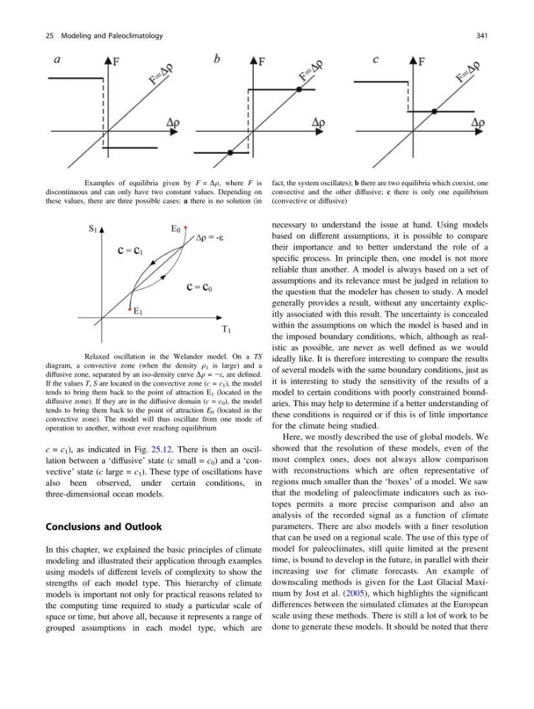
Fig. 25.11 Examples of equilibria given by F = Dq, where F is
discontinuous and can only have two constant values. Depending on
these values, there are three possible cases: a there is no solution (in
fact, the system oscillates); b there are two equilibria which coexist, one
convective and the other diffusive; c there is only one equilibrium
(convective or diffusive)
Fig. 25.12 Relaxed oscillation in the Welander model. On a TS
diagram, a convective zone (when the density q 1 is large) and a
diffusive zone, separated by an iso-density curve Dq = −e, are defined.
If the values T, S are located in the convective zone (c = c 1 ), the model
tends to bring them back to the point of attraction E 1 (located in the
diffusive zone). If they are in the diffusive domain (c = c 0 ), the model
tends to bring them back to the point of attraction E 0 (located in the
convective zone). The model will thus oscillate from one mode of
operation to another, without ever reaching equilibrium
25 Modeling and Paleoclimatology
341
also been observed, under certain conditions, in
three-dimensional ocean models.
Conclusions and Outlook
In this chapter, we explained the basic principles of climate
modeling and illustrated their application through examples
using models of different levels of complexity to show the
strengths of each model type. This hierarchy of climate
models is important not only for practical reasons related to
the computing time required to study a particular scale of
space or time, but above all, because it represents a range of
grouped assumptions in each model type, which are
necessary to understand the issue at hand. Using models
based on different assumptions, it is possible to compare
their importance and to better understand the role of a
specific process. In principle then, one model is not more
reliable than another. A model is always based on a set of
assumptions and its relevance must be judged in relation to
the question that the modeler has chosen to study. A model
generally provides a result, without any uncertainty explicitly associated with this result. The uncertainty is concealed
within the assumptions on which the model is based and in
the imposed boundary conditions, which, although as realistic as possible, are never as well defined as we would
ideally like. It is therefore interesting to compare the results
of several models with the same boundary conditions, just as
it is interesting to study the sensitivity of the results of a
model to certain conditions with poorly constrained boundaries. This may help to determine if a better understanding of
these conditions is required or if this is of little importance
for the climate being studied.
Here, we mostly described the use of global models. We
showed that the resolution of these models, even of the
most complex ones, does not always allow comparison
with reconstructions which are often representative of
regions much smaller than the ‘boxes’ of a model. We saw
that the modeling of paleoclimate indicators such as isotopes permits a more precise comparison and also an
analysis of the recorded signal as a function of climate
parameters. There are also models with a finer resolution
that can be used on a regional scale. The use of this type of
model for paleoclimates, still quite limited at the present
time, is bound to develop in the future, in parallel with their
increasing use for climate forecasts. An example of
downscaling methods is given for the Last Glacial Maximum by Jost et al. (2005), which highlights the significant
differences between the simulated climates at the European
scale using these methods. There is still a lot of work to be
done to generate these models. It should be noted that there
Fig. 25.11 Examples of equilibria given by F = Dq, where F is
discontinuous and can only have two constant values. Depending on
these values, there are three possible cases: a there is no solution (in
fact, the system oscillates); b there are two equilibria which coexist, one
convective and the other diffusive; c there is only one equilibrium
(convective or diffusive)
Fig. 25.12 Relaxed oscillation in the Welander model. On a TS
diagram, a convective zone (when the density q 1 is large) and a
diffusive zone, separated by an iso-density curve Dq = −e, are defined.
If the values T, S are located in the convective zone (c = c 1 ), the model
tends to bring them back to the point of attraction E 1 (located in the
diffusive zone). If they are in the diffusive domain (c = c 0 ), the model
tends to bring them back to the point of attraction E 0 (located in the
convective zone). The model will thus oscillate from one mode of
operation to another, without ever reaching equilibrium
25 Modeling and Paleoclimatology
341