

The equilibrium is stable when any infinitesimal increase
in the salinity gradient DS leads to an increase in the term |
m|DS, so that the derivative of DS relative to time becomes
slightly negative. The direction of variation of |m|DS as a
function of DS is in fact given directly by the figure representing |1 − x|x as a function of x. The descending intermediate branch (dashed line in the figure) indicates a
decrease in |m|DS when DS increases, leading to an unstable
equilibrium. The ‘thermal’ and ‘saline’ branches, on the
other hand, are perfectly stable. For the same value of the
temperatures and the salt flux, there are therefore two stable
equilibria possible in this system.
Interestingly, these multiple equilibria are found in much
more complex models of the ocean, and even in some
ocean-atmosphere coupled models (Rahmstorf 1996;
Rahmstorf et al. 2005). It therefore seems that this very
simple model captures an important aspect of thermohaline
circulation, which explains the existence of sudden variations in the deep ocean circulation. These variations are most
likely involved in the sudden climate changes observed
during the ice ages (Heinrich events and DansgaardOeschger events, see Chap. 29).
The Welander Model
The multiplicity of equilibria does not explain everything,
and of course there are other types of possible behaviors.
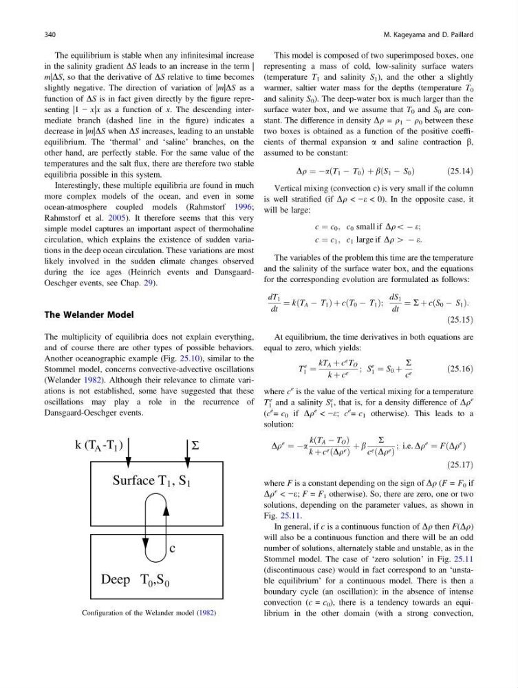
Another oceanographic example (Fig. 25.10), similar to the
Stommel model, concerns convective-advective oscillations
(Welander 1982). Although their relevance to climate variations is not established, some have suggested that these
oscillations may play a role in the recurrence of
Dansgaard-Oeschger events.
This model is composed of two superimposed boxes, one
representing a mass of cold, low-salinity surface waters
(temperature T 1 and salinity S 1 ), and the other a slightly
warmer, saltier water mass for the depths (temperature T 0
and salinity S 0 ). The deep-water box is much larger than the
surface water box, and we assume that T 0 and S 0 are constant. The difference in density Dq = q 1 − q 0 between these
two boxes is obtained as a function of the positive coefficients of thermal expansion a and saline contraction b,
assumed to be constant:
Dq ¼ ÀaðT 1 À T 0 Þ þ bðS 1 À S 0 Þ
ð 25:14Þ
Vertical mixing (convection c) is very small if the column
is well stratified (if Dq < −e < 0). In the opposite case, it
will be large:
c ¼ c 0 ; c 0 small if Dq\ À e;
c ¼ c 1 ; c 1 large if Dq [ À e:
The variables of the problem this time are the temperature
and the salinity of the surface water box, and the equations
for the corresponding evolution are formulated as follows:
dT 1
dt
¼ kðT A À T 1 Þ þ cðT 0 À T 1 Þ;
dS 1
dt
¼ R þ cðS 0 À S 1 Þ:
ð25:15Þ
At equilibrium, the time derivatives in both equations are
equal to zero, which yields:
T
e
1 ¼
kT A þ c
e T O
k þ c e ; S
e
1 ¼ S 0 þ
R
c e
ð25:16Þ
where c
e is the value of the vertical mixing for a temperature
T
e
1 and a salinity S
e
1 , that is, for a density difference of Dq
e
(c
e = c 0 if Dq
e < −e; c
e = c 1 otherwise). This leads to a
solution:
Dq
e
¼ Àa
k T A À T O
ð
Þ
k þ c e Dq e
ð
Þ
þ b
R
c e Dq e
ð
Þ
; i.e. Dq
e
¼ F Dq
e
ð
Þ
ð25:17Þ
where F is a constant depending on the sign of Dq (F = F 0 if
Dq
e < −e; F = F 1 otherwise). So, there are zero, one or two
solutions, depending on the parameter values, as shown in
Fig. 25.11.
In general, if c is a continuous function of Dq then F(Dq)
will also be a continuous function and there will be an odd
number of solutions, alternately stable and unstable, as in the
Stommel model. The case of ‘zero solution’ in Fig. 25.11
(discontinuous case) would in fact correspond to an ‘unstable equilibrium’ for a continuous model. There is then a
boundary cycle (an oscillation): in the absence of intense
convection (c = c 0 ), there is a tendency towards an equilibrium in the other domain (with a strong convection,
Surface T 1 , S 1
c
Deep T 0 ,S 0
k (T A -T 1 )
Σ
Fig. 25.10 Configuration of the Welander model (1982)
340
M. Kageyama and D. Paillard
in the salinity gradient DS leads to an increase in the term |
m|DS, so that the derivative of DS relative to time becomes
slightly negative. The direction of variation of |m|DS as a
function of DS is in fact given directly by the figure representing |1 − x|x as a function of x. The descending intermediate branch (dashed line in the figure) indicates a
decrease in |m|DS when DS increases, leading to an unstable
equilibrium. The ‘thermal’ and ‘saline’ branches, on the
other hand, are perfectly stable. For the same value of the
temperatures and the salt flux, there are therefore two stable
equilibria possible in this system.
Interestingly, these multiple equilibria are found in much
more complex models of the ocean, and even in some
ocean-atmosphere coupled models (Rahmstorf 1996;
Rahmstorf et al. 2005). It therefore seems that this very
simple model captures an important aspect of thermohaline
circulation, which explains the existence of sudden variations in the deep ocean circulation. These variations are most
likely involved in the sudden climate changes observed
during the ice ages (Heinrich events and DansgaardOeschger events, see Chap. 29).
The Welander Model
The multiplicity of equilibria does not explain everything,
and of course there are other types of possible behaviors.
Another oceanographic example (Fig. 25.10), similar to the
Stommel model, concerns convective-advective oscillations
(Welander 1982). Although their relevance to climate variations is not established, some have suggested that these
oscillations may play a role in the recurrence of
Dansgaard-Oeschger events.
This model is composed of two superimposed boxes, one
representing a mass of cold, low-salinity surface waters
(temperature T 1 and salinity S 1 ), and the other a slightly
warmer, saltier water mass for the depths (temperature T 0
and salinity S 0 ). The deep-water box is much larger than the
surface water box, and we assume that T 0 and S 0 are constant. The difference in density Dq = q 1 − q 0 between these
two boxes is obtained as a function of the positive coefficients of thermal expansion a and saline contraction b,
assumed to be constant:
Dq ¼ ÀaðT 1 À T 0 Þ þ bðS 1 À S 0 Þ
ð 25:14Þ
Vertical mixing (convection c) is very small if the column
is well stratified (if Dq < −e < 0). In the opposite case, it
will be large:
c ¼ c 0 ; c 0 small if Dq\ À e;
c ¼ c 1 ; c 1 large if Dq [ À e:
The variables of the problem this time are the temperature
and the salinity of the surface water box, and the equations
for the corresponding evolution are formulated as follows:
dT 1
dt
¼ kðT A À T 1 Þ þ cðT 0 À T 1 Þ;
dS 1
dt
¼ R þ cðS 0 À S 1 Þ:
ð25:15Þ
At equilibrium, the time derivatives in both equations are
equal to zero, which yields:
T
e
1 ¼
kT A þ c
e T O
k þ c e ; S
e
1 ¼ S 0 þ
R
c e
ð25:16Þ
where c
e is the value of the vertical mixing for a temperature
T
e
1 and a salinity S
e
1 , that is, for a density difference of Dq
e
(c
e = c 0 if Dq
e < −e; c
e = c 1 otherwise). This leads to a
solution:
Dq
e
¼ Àa
k T A À T O
ð
Þ
k þ c e Dq e
ð
Þ
þ b
R
c e Dq e
ð
Þ
; i.e. Dq
e
¼ F Dq
e
ð
Þ
ð25:17Þ
where F is a constant depending on the sign of Dq (F = F 0 if
Dq
e < −e; F = F 1 otherwise). So, there are zero, one or two
solutions, depending on the parameter values, as shown in
Fig. 25.11.
In general, if c is a continuous function of Dq then F(Dq)
will also be a continuous function and there will be an odd
number of solutions, alternately stable and unstable, as in the
Stommel model. The case of ‘zero solution’ in Fig. 25.11
(discontinuous case) would in fact correspond to an ‘unstable equilibrium’ for a continuous model. There is then a
boundary cycle (an oscillation): in the absence of intense
convection (c = c 0 ), there is a tendency towards an equilibrium in the other domain (with a strong convection,
Surface T 1 , S 1
c
Deep T 0 ,S 0
k (T A -T 1 )
Σ
Fig. 25.10 Configuration of the Welander model (1982)
340
M. Kageyama and D. Paillard