

Dq ¼ Àa T 2 À T 1
ð
Þþb S 2 À S 1
ð
Þ
ð 25:8Þ
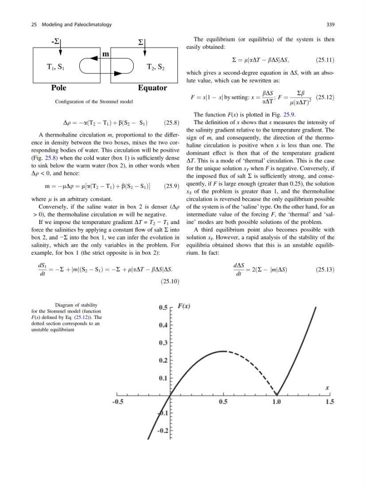
A thermohaline circulation m, proportional to the difference in density between the two boxes, mixes the two corresponding bodies of water. This circulation will be positive
(Fig. 25.8) when the cold water (box 1) is sufficiently dense
to sink below the warm water (box 2), in other words when
Dq < 0, and hence:
m ¼ ÀlDq ¼ l a T 2 À T 1
ð
Þþb S 2 À S 1
ð
Þ
½
ð 25:9Þ
where l is an arbitrary constant.
Conversely, if the saline water in box 2 is denser (Dq
> 0), the thermohaline circulation m will be negative.
If we impose the temperature gradient DT = T 2 − T 1 and
force the salinities by applying a constant flow of salt R into
box 2, and −R into the box 1, we can infer the evolution in
salinity, which are the only variables in the problem. For
example, for box 1 (the strict opposite is in box 2):
dS 1
dt
¼ ÀR þ m
j j S 2 À S 1
ð
Þ¼À R þ l aDT À bDS
j
j DS:
ð25:10Þ
The equilibrium (or equilibria) of the system is then
easily obtained:
R ¼ l aDT À bDS
j
j DS;
ð25:11Þ
which gives a second-degree equation in DS, with an absolute value, which can be rewritten as:
F ¼ x 1 À x
j
jby setting: x ¼
bDS
aDT
; F ¼
Rb
l aDT
ð
Þ
2
ð25:12Þ
The function F(x) is plotted in Fig. 25.9.
The definition of x shows that x measures the intensity of
the salinity gradient relative to the temperature gradient. The
sign of m, and consequently, the direction of the thermohaline circulation is positive when x is less than one. The
dominant effect is then that of the temperature gradient
DT. This is a mode of ‘thermal’ circulation. This is the case
for the unique solution x T when F is negative. Conversely, if
the imposed flux of salt R is sufficiently strong, and consequently, if F is large enough (greater than 0.25), the solution
x S of the problem is greater than 1, and the thermohaline
circulation is reversed because the only equilibrium possible
of the system is of the ‘saline’ type. On the other hand, for an
intermediate value of the forcing F, the ‘thermal’ and ‘saline’ modes are both possible solutions of the problem.
A third equilibrium point also becomes possible with
solution x I . However, a rapid analysis of the stability of the
equilibria obtained shows that this is an unstable equilibrium. In fact:
dDS
dt
¼ 2ðR À m
j jDSÞ
ð 25:13Þ
T 1 , S 1
T 2 , S 2
m
Pole
-Σ
Σ
Equator
Fig. 25.8 Configuration of the Stommel model
Fig. 25.9 Diagram of stability
for the Stommel model (function
F(x) defined by Eq. (25.12)). The
dotted section corresponds to an
unstable equilibrium
25 Modeling and Paleoclimatology
339
ð
Þþb S 2 À S 1
ð
Þ
ð 25:8Þ
A thermohaline circulation m, proportional to the difference in density between the two boxes, mixes the two corresponding bodies of water. This circulation will be positive
(Fig. 25.8) when the cold water (box 1) is sufficiently dense
to sink below the warm water (box 2), in other words when
Dq < 0, and hence:
m ¼ ÀlDq ¼ l a T 2 À T 1
ð
Þþb S 2 À S 1
ð
Þ
½
ð 25:9Þ
where l is an arbitrary constant.
Conversely, if the saline water in box 2 is denser (Dq
> 0), the thermohaline circulation m will be negative.
If we impose the temperature gradient DT = T 2 − T 1 and
force the salinities by applying a constant flow of salt R into
box 2, and −R into the box 1, we can infer the evolution in
salinity, which are the only variables in the problem. For
example, for box 1 (the strict opposite is in box 2):
dS 1
dt
¼ ÀR þ m
j j S 2 À S 1
ð
Þ¼À R þ l aDT À bDS
j
j DS:
ð25:10Þ
The equilibrium (or equilibria) of the system is then
easily obtained:
R ¼ l aDT À bDS
j
j DS;
ð25:11Þ
which gives a second-degree equation in DS, with an absolute value, which can be rewritten as:
F ¼ x 1 À x
j
jby setting: x ¼
bDS
aDT
; F ¼
Rb
l aDT
ð
Þ
2
ð25:12Þ
The function F(x) is plotted in Fig. 25.9.
The definition of x shows that x measures the intensity of
the salinity gradient relative to the temperature gradient. The
sign of m, and consequently, the direction of the thermohaline circulation is positive when x is less than one. The
dominant effect is then that of the temperature gradient
DT. This is a mode of ‘thermal’ circulation. This is the case
for the unique solution x T when F is negative. Conversely, if
the imposed flux of salt R is sufficiently strong, and consequently, if F is large enough (greater than 0.25), the solution
x S of the problem is greater than 1, and the thermohaline
circulation is reversed because the only equilibrium possible
of the system is of the ‘saline’ type. On the other hand, for an
intermediate value of the forcing F, the ‘thermal’ and ‘saline’ modes are both possible solutions of the problem.
A third equilibrium point also becomes possible with
solution x I . However, a rapid analysis of the stability of the
equilibria obtained shows that this is an unstable equilibrium. In fact:
dDS
dt
¼ 2ðR À m
j jDSÞ
ð 25:13Þ
T 1 , S 1
T 2 , S 2
m
Pole
-Σ
Σ
Equator
Fig. 25.8 Configuration of the Stommel model
Fig. 25.9 Diagram of stability
for the Stommel model (function
F(x) defined by Eq. (25.12)). The
dotted section corresponds to an
unstable equilibrium
25 Modeling and Paleoclimatology
339