

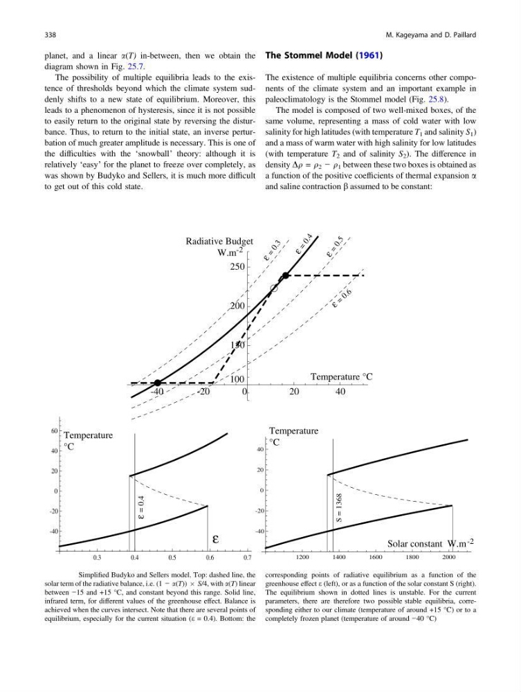
planet, and a linear a(T) in-between, then we obtain the
diagram shown in Fig. 25.7.
The possibility of multiple equilibria leads to the existence of thresholds beyond which the climate system suddenly shifts to a new state of equilibrium. Moreover, this
leads to a phenomenon of hysteresis, since it is not possible
to easily return to the original state by reversing the disturbance. Thus, to return to the initial state, an inverse perturbation of much greater amplitude is necessary. This is one of
the difficulties with the ‘snowball’ theory: although it is
relatively ‘easy’ for the planet to freeze over completely, as
was shown by Budyko and Sellers, it is much more difficult
to get out of this cold state.
The Stommel Model (1961)
The existence of multiple equilibria concerns other components of the climate system and an important example in
paleoclimatology is the Stommel model (Fig. 25.8).
The model is composed of two well-mixed boxes, of the
same volume, representing a mass of cold water with low
salinity for high latitudes (with temperature T 1 and salinity S 1 )
and a mass of warm water with high salinity for low latitudes
(with temperature T 2 and of salinity S 2 ). The difference in
density Dq = q 2 − q 1 between these two boxes is obtained as
a function of the positive coefficients of thermal expansion a
and saline contraction b assumed to be constant:
-40
-20
20
40
150
200
250
Radiative Budget
W.m -2
0
100
Temperature °C
ε = 0 . 4
ε = 0 . 3
ε = 0 . 5
ε
=
0 . 6
0.3
0.4
0.5
0.6
0.7
-40
-20
0
20
40
60
1200
1400
1600
1800
2000
-40
-20
0
20
40
ε
Temperature
°C
Temperature
°C
ε 4
.
0
=
Solar constant W.m -2
8
6
3
1
=
S
Fig. 25.7 Simplified Budyko and Sellers model. Top: dashed line, the
solar term of the radiative balance, i.e. (1 − a(T)) Â S/4, with a(T) linear
between −15 and +15 °C, and constant beyond this range. Solid line,
infrared term, for different values of the greenhouse effect. Balance is
achieved when the curves intersect. Note that there are several points of
equilibrium, especially for the current situation (e = 0.4). Bottom: the
corresponding points of radiative equilibrium as a function of the
greenhouse effect e (left), or as a function of the solar constant S (right).
The equilibrium shown in dotted lines is unstable. For the current
parameters, there are therefore two possible stable equilibria, corresponding either to our climate (temperature of around +15 °C) or to a
completely frozen planet (temperature of around −40 °C)
338
M. Kageyama and D. Paillard
diagram shown in Fig. 25.7.
The possibility of multiple equilibria leads to the existence of thresholds beyond which the climate system suddenly shifts to a new state of equilibrium. Moreover, this
leads to a phenomenon of hysteresis, since it is not possible
to easily return to the original state by reversing the disturbance. Thus, to return to the initial state, an inverse perturbation of much greater amplitude is necessary. This is one of
the difficulties with the ‘snowball’ theory: although it is
relatively ‘easy’ for the planet to freeze over completely, as
was shown by Budyko and Sellers, it is much more difficult
to get out of this cold state.
The Stommel Model (1961)
The existence of multiple equilibria concerns other components of the climate system and an important example in
paleoclimatology is the Stommel model (Fig. 25.8).
The model is composed of two well-mixed boxes, of the
same volume, representing a mass of cold water with low
salinity for high latitudes (with temperature T 1 and salinity S 1 )
and a mass of warm water with high salinity for low latitudes
(with temperature T 2 and of salinity S 2 ). The difference in
density Dq = q 2 − q 1 between these two boxes is obtained as
a function of the positive coefficients of thermal expansion a
and saline contraction b assumed to be constant:
-40
-20
20
40
150
200
250
Radiative Budget
W.m -2
0
100
Temperature °C
ε = 0 . 4
ε = 0 . 3
ε = 0 . 5
ε
=
0 . 6
0.3
0.4
0.5
0.6
0.7
-40
-20
0
20
40
60
1200
1400
1600
1800
2000
-40
-20
0
20
40
ε
Temperature
°C
Temperature
°C
ε 4
.
0
=
Solar constant W.m -2
8
6
3
1
=
S
Fig. 25.7 Simplified Budyko and Sellers model. Top: dashed line, the
solar term of the radiative balance, i.e. (1 − a(T)) Â S/4, with a(T) linear
between −15 and +15 °C, and constant beyond this range. Solid line,
infrared term, for different values of the greenhouse effect. Balance is
achieved when the curves intersect. Note that there are several points of
equilibrium, especially for the current situation (e = 0.4). Bottom: the
corresponding points of radiative equilibrium as a function of the
greenhouse effect e (left), or as a function of the solar constant S (right).
The equilibrium shown in dotted lines is unstable. For the current
parameters, there are therefore two possible stable equilibria, corresponding either to our climate (temperature of around +15 °C) or to a
completely frozen planet (temperature of around −40 °C)
338
M. Kageyama and D. Paillard