

difference in global temperature due to a doubling of CO 2 ,
see Chap. 31). The current climate, as defined by the
observations, makes it possible to make a first choice of
parameters so that an acceptable simulated climate can be
achieved. The authors show that reconstructions of tropical
temperatures during the Last Glacial Maximum help to
constrain even further the selection of values of these
parameters and so reduce the uncertainties associated with
future climate change. This study shows that modeling of
past climates followed by comparison with reconstructions
can help in the evaluation of climate models used to forecast
future climate. This conclusion is also advanced by Hargreaves et al. (2007) using a general circulation model.
Outlook
It might be expected that with the advances in computing,
climate models of intermediate complexity would no longer
have any reason to exist. In fact, this is not the case because
they will always be less time consuming than general circulation models, which incorporate more and more mechanisms
and use an increasingly fine resolution. In some ways, general
circulation models, such as those used for IPCC simulations,
are defined by the capabilities of the most powerful computers. We need to be able to use these models to produce
simulations of several hundred years within a reasonable time
on available computers. Long simulations, necessary to
understand past climate changes reconstructed using multiple
indicators and the need to explore different scenarios and
model parameters, require faster models. Today’s general
circulation models will no doubt become the intermediate
complexity models of tomorrow, but this concept will continue to exist. In addition, it is important to retain this hierarchy of models because each type of model is established on
different assumptions. By comparing the results of different
models, it is possible to highlight the relative importance of a
particular process which is included in one model but not in
the other or which is represented differently in each model.
Conceptual Models
The main objective of the models described above is to try to
reproduce the observations we have for the climate system
and its variations in the past. As has been highlighted,
modeling also aims to improve our understanding of these
variations, and it is therefore useful to describe some aspects
of the system using extremely simple models, which are
intended to illustrate some key processes. These are called
conceptual models. There are many varied examples. One
example is the Lorenz model (Fig. 25.1d), which often serves
as an archetype of the chaotic system. The meteorologist
Edward Lorenz proposed a very simple model, based on an
idealized thermal convection, which for the first time illustrated that the complexity of the behavior of a dynamic
system was absolutely unrelated to the number of degrees of
freedom of this system, as many previously imagined. He
showed that a very simple system (in this case with only three
degrees of freedom) can produce unpredictable behavior,
called ‘deterministic chaos’. This conceptual model still
plays an important educational role, and its mathematical
properties are still a subject of active research. Below, some
examples directly relevant to the climate system are described in more detail. Other examples, shown in Chap. 28, aim
to achieve a better understanding of the glacial-interglacial
dynamics (Calder, Imbrie models etc.).
The Budyko/Sellers Model
The Earth’s climate is determined above all by its radiative
balance. By simulating simplified balances, it is possible to
estimate the magnitude of a change in temperature caused
by, for example, changes in the incident solar radiation
(volcanic dust, changes in the solar constant, nuclear winter,
etc.). In 1969, two publications (Budyko 1969, Sellers 1969)
came to a somewhat surprising conclusion: if we take
account of the feedback between temperature and albedo, a
relatively small decrease in the solar constant (−1.5% or
−2%) is enough for the Earth to completely freeze over.
A similar result also occurs when the greenhouse effect is
modified. This indicates that there is a critical threshold
towards cooling which causes the climate system to move
into a very different state. The meaning of these results has
now become even more pertinent with the theory of Snowball Earth (Chap. 26).
In their original versions, Budyko’s and Sellers’ models
are explicitly dependent on latitude and predict a temperature T(y) where y is the latitude. A much simpler version can
be formulated to represent the phenomenon of runaway
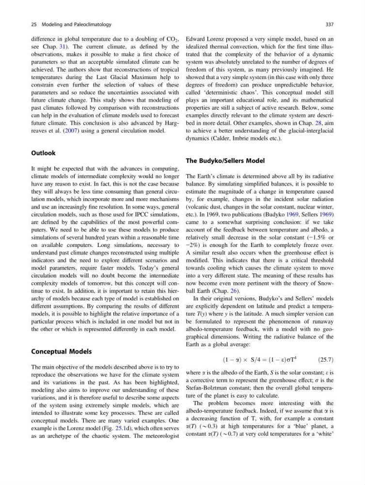
albedo-temperature feedback, with a model with no geographical dimensions. Writing the radiative balance of the
Earth as a global average:
1 À a
ð
ÞÂ S=4 ¼ 1 À e
ð
ÞrT
4
ð25:7Þ
where a is the albedo of the Earth, S is the solar constant; e is
a corrective term to represent the greenhouse effect; r is the
Stefan-Bolztman constant; then the overall global temperature of the planet is easy to calculate.
The problem becomes more interesting with the
albedo-temperature feedback. Indeed, if we assume that a is
a decreasing function of T, with, for example a constant
a(T) (*0.3) at high temperatures for a ‘blue’ planet, a
constant a(T) (*0.7) at very cold temperatures for a ‘white’
25 Modeling and Paleoclimatology
337
see Chap. 31). The current climate, as defined by the
observations, makes it possible to make a first choice of
parameters so that an acceptable simulated climate can be
achieved. The authors show that reconstructions of tropical
temperatures during the Last Glacial Maximum help to
constrain even further the selection of values of these
parameters and so reduce the uncertainties associated with
future climate change. This study shows that modeling of
past climates followed by comparison with reconstructions
can help in the evaluation of climate models used to forecast
future climate. This conclusion is also advanced by Hargreaves et al. (2007) using a general circulation model.
Outlook
It might be expected that with the advances in computing,
climate models of intermediate complexity would no longer
have any reason to exist. In fact, this is not the case because
they will always be less time consuming than general circulation models, which incorporate more and more mechanisms
and use an increasingly fine resolution. In some ways, general
circulation models, such as those used for IPCC simulations,
are defined by the capabilities of the most powerful computers. We need to be able to use these models to produce
simulations of several hundred years within a reasonable time
on available computers. Long simulations, necessary to
understand past climate changes reconstructed using multiple
indicators and the need to explore different scenarios and
model parameters, require faster models. Today’s general
circulation models will no doubt become the intermediate
complexity models of tomorrow, but this concept will continue to exist. In addition, it is important to retain this hierarchy of models because each type of model is established on
different assumptions. By comparing the results of different
models, it is possible to highlight the relative importance of a
particular process which is included in one model but not in
the other or which is represented differently in each model.
Conceptual Models
The main objective of the models described above is to try to
reproduce the observations we have for the climate system
and its variations in the past. As has been highlighted,
modeling also aims to improve our understanding of these
variations, and it is therefore useful to describe some aspects
of the system using extremely simple models, which are
intended to illustrate some key processes. These are called
conceptual models. There are many varied examples. One
example is the Lorenz model (Fig. 25.1d), which often serves
as an archetype of the chaotic system. The meteorologist
Edward Lorenz proposed a very simple model, based on an
idealized thermal convection, which for the first time illustrated that the complexity of the behavior of a dynamic
system was absolutely unrelated to the number of degrees of
freedom of this system, as many previously imagined. He
showed that a very simple system (in this case with only three
degrees of freedom) can produce unpredictable behavior,
called ‘deterministic chaos’. This conceptual model still
plays an important educational role, and its mathematical
properties are still a subject of active research. Below, some
examples directly relevant to the climate system are described in more detail. Other examples, shown in Chap. 28, aim
to achieve a better understanding of the glacial-interglacial
dynamics (Calder, Imbrie models etc.).
The Budyko/Sellers Model
The Earth’s climate is determined above all by its radiative
balance. By simulating simplified balances, it is possible to
estimate the magnitude of a change in temperature caused
by, for example, changes in the incident solar radiation
(volcanic dust, changes in the solar constant, nuclear winter,
etc.). In 1969, two publications (Budyko 1969, Sellers 1969)
came to a somewhat surprising conclusion: if we take
account of the feedback between temperature and albedo, a
relatively small decrease in the solar constant (−1.5% or
−2%) is enough for the Earth to completely freeze over.
A similar result also occurs when the greenhouse effect is
modified. This indicates that there is a critical threshold
towards cooling which causes the climate system to move
into a very different state. The meaning of these results has
now become even more pertinent with the theory of Snowball Earth (Chap. 26).
In their original versions, Budyko’s and Sellers’ models
are explicitly dependent on latitude and predict a temperature T(y) where y is the latitude. A much simpler version can
be formulated to represent the phenomenon of runaway
albedo-temperature feedback, with a model with no geographical dimensions. Writing the radiative balance of the
Earth as a global average:
1 À a
ð
ÞÂ S=4 ¼ 1 À e
ð
ÞrT
4
ð25:7Þ
where a is the albedo of the Earth, S is the solar constant; e is
a corrective term to represent the greenhouse effect; r is the
Stefan-Bolztman constant; then the overall global temperature of the planet is easy to calculate.
The problem becomes more interesting with the
albedo-temperature feedback. Indeed, if we assume that a is
a decreasing function of T, with, for example a constant
a(T) (*0.3) at high temperatures for a ‘blue’ planet, a
constant a(T) (*0.7) at very cold temperatures for a ‘white’
25 Modeling and Paleoclimatology
337