

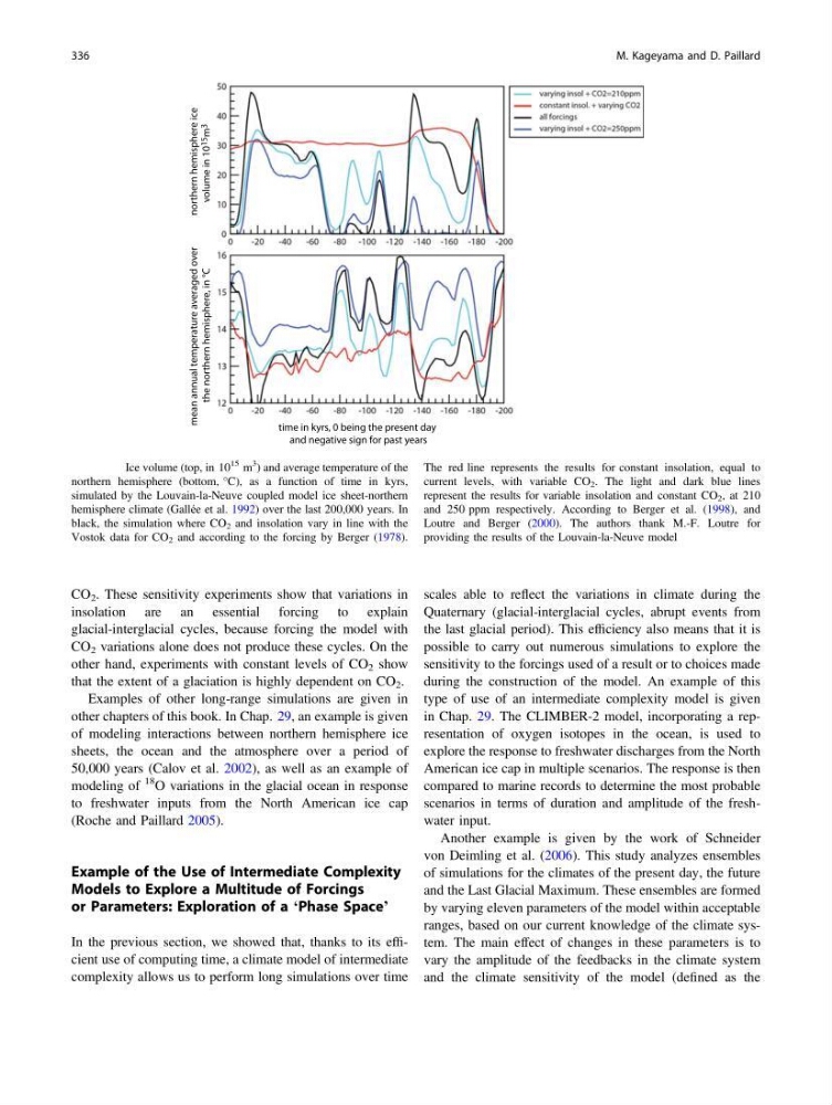
CO 2 . These sensitivity experiments show that variations in
insolation are an essential forcing to explain
glacial-interglacial cycles, because forcing the model with
CO 2 variations alone does not produce these cycles. On the
other hand, experiments with constant levels of CO 2 show
that the extent of a glaciation is highly dependent on CO 2 .
Examples of other long-range simulations are given in
other chapters of this book. In Chap. 29, an example is given
of modeling interactions between northern hemisphere ice
sheets, the ocean and the atmosphere over a period of
50,000 years (Calov et al. 2002), as well as an example of
modeling of
18 O variations in the glacial ocean in response
to freshwater inputs from the North American ice cap
(Roche and Paillard 2005).
Example of the Use of Intermediate Complexity
Models to Explore a Multitude of Forcings
or Parameters: Exploration of a ‘Phase Space’
In the previous section, we showed that, thanks to its efficient use of computing time, a climate model of intermediate
complexity allows us to perform long simulations over time
scales able to reflect the variations in climate during the
Quaternary (glacial-interglacial cycles, abrupt events from
the last glacial period). This efficiency also means that it is
possible to carry out numerous simulations to explore the
sensitivity to the forcings used of a result or to choices made
during the construction of the model. An example of this
type of use of an intermediate complexity model is given
in Chap. 29. The CLIMBER-2 model, incorporating a representation of oxygen isotopes in the ocean, is used to
explore the response to freshwater discharges from the North
American ice cap in multiple scenarios. The response is then
compared to marine records to determine the most probable
scenarios in terms of duration and amplitude of the freshwater input.
Another example is given by the work of Schneider
von Deimling et al. (2006). This study analyzes ensembles
of simulations for the climates of the present day, the future
and the Last Glacial Maximum. These ensembles are formed
by varying eleven parameters of the model within acceptable
ranges, based on our current knowledge of the climate system. The main effect of changes in these parameters is to
vary the amplitude of the feedbacks in the climate system
and the climate sensitivity of the model (defined as the
northern hemisphere ice
volume in 10 15
m 3
mean annual temperature averaged over
the northern hemisphere, in °C
time in kyrs, 0 being the present day
and negative sign for past years
Fig. 25.6 Ice volume (top, in 10
15 m
3
) and average temperature of the
northern hemisphere (bottom, °C), as a function of time in kyrs,
simulated by the Louvain-la-Neuve coupled model ice sheet-northern
hemisphere climate (Gallée et al. 1992) over the last 200,000 years. In
black, the simulation where CO 2 and insolation vary in line with the
Vostok data for CO 2 and according to the forcing by Berger (1978).
The red line represents the results for constant insolation, equal to
current levels, with variable CO 2 . The light and dark blue lines
represent the results for variable insolation and constant CO 2 , at 210
and 250 ppm respectively. According to Berger et al. (1998), and
Loutre and Berger (2000). The authors thank M.-F. Loutre for
providing the results of the Louvain-la-Neuve model
336
M. Kageyama and D. Paillard
insolation are an essential forcing to explain
glacial-interglacial cycles, because forcing the model with
CO 2 variations alone does not produce these cycles. On the
other hand, experiments with constant levels of CO 2 show
that the extent of a glaciation is highly dependent on CO 2 .
Examples of other long-range simulations are given in
other chapters of this book. In Chap. 29, an example is given
of modeling interactions between northern hemisphere ice
sheets, the ocean and the atmosphere over a period of
50,000 years (Calov et al. 2002), as well as an example of
modeling of
18 O variations in the glacial ocean in response
to freshwater inputs from the North American ice cap
(Roche and Paillard 2005).
Example of the Use of Intermediate Complexity
Models to Explore a Multitude of Forcings
or Parameters: Exploration of a ‘Phase Space’
In the previous section, we showed that, thanks to its efficient use of computing time, a climate model of intermediate
complexity allows us to perform long simulations over time
scales able to reflect the variations in climate during the
Quaternary (glacial-interglacial cycles, abrupt events from
the last glacial period). This efficiency also means that it is
possible to carry out numerous simulations to explore the
sensitivity to the forcings used of a result or to choices made
during the construction of the model. An example of this
type of use of an intermediate complexity model is given
in Chap. 29. The CLIMBER-2 model, incorporating a representation of oxygen isotopes in the ocean, is used to
explore the response to freshwater discharges from the North
American ice cap in multiple scenarios. The response is then
compared to marine records to determine the most probable
scenarios in terms of duration and amplitude of the freshwater input.
Another example is given by the work of Schneider
von Deimling et al. (2006). This study analyzes ensembles
of simulations for the climates of the present day, the future
and the Last Glacial Maximum. These ensembles are formed
by varying eleven parameters of the model within acceptable
ranges, based on our current knowledge of the climate system. The main effect of changes in these parameters is to
vary the amplitude of the feedbacks in the climate system
and the climate sensitivity of the model (defined as the
northern hemisphere ice
volume in 10 15
m 3
mean annual temperature averaged over
the northern hemisphere, in °C
time in kyrs, 0 being the present day
and negative sign for past years
Fig. 25.6 Ice volume (top, in 10
15 m
3
) and average temperature of the
northern hemisphere (bottom, °C), as a function of time in kyrs,
simulated by the Louvain-la-Neuve coupled model ice sheet-northern
hemisphere climate (Gallée et al. 1992) over the last 200,000 years. In
black, the simulation where CO 2 and insolation vary in line with the
Vostok data for CO 2 and according to the forcing by Berger (1978).
The red line represents the results for constant insolation, equal to
current levels, with variable CO 2 . The light and dark blue lines
represent the results for variable insolation and constant CO 2 , at 210
and 250 ppm respectively. According to Berger et al. (1998), and
Loutre and Berger (2000). The authors thank M.-F. Loutre for
providing the results of the Louvain-la-Neuve model
336
M. Kageyama and D. Paillard