

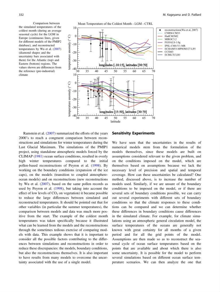
Ramstein et al. (2007) summarized the efforts of the years
2000’s to reach a congruent comparison between reconstructions and simulations for winter temperatures during the
Last Glacial Maximum. The simulations of the PMIP1
project, using standalone atmospheric models forced by the
CLIMAP (1981) ocean surface conditions, resulted in overly
high winter temperatures compared to the initial
pollen-based reconstructions of Peyron et al. (1998). By
working on the boundary conditions (expansion of the ice
caps), on the models (transition to coupled atmosphereocean models) and on reconstructions (new reconstructions
by Wu et al. (2007), based on the same pollen records as
used by Peyron et al. (1998), but taking into account the
effect of low levels of CO 2 on vegetation) it became possible
to reduce the large differences between simulated and
reconstructed temperatures. It should be pointed out that for
other variables (in particular the summer temperatures), the
comparison between models and data was much more positive from the start. The example of the coldest month
temperatures was taken specifically because it illustrated
what can be learned from the models and the reconstructions
through the sometimes tedious exercise of comparing models with data. This example shows that it is important to
consider all the possible factors contributing to the differences between simulations and reconstructions in order to
reduce these discrepancies: the models, boundary conditions,
but also the reconstructions themselves. It is also important
to have results from many models to overcome the uncertainty associated with the use of a single model.
Sensitivity Experiments
We have seen that the uncertainties in the results of
numerical models stem from the formulation of the
models themselves, since these models are built on
assumptions considered relevant to the given problem, and
on the conditions imposed on the model, which are
themselves based on assumptions because we lack the
necessary level of precision and spatial and temporal
coverage. How can these uncertainties be calculated? One
method, discussed above, is to increase the number of
models used. Similarly, if we are unsure of the boundary
conditions to be imposed on the model, or if there are
several sets of boundary conditions possible, we can carry
out several experiments with different sets of boundary
conditions so that the climate responses to these conditions can be compared and we can determine whether
these differences in boundary conditions cause differences
in the simulated climate. For example, for climate simulations using an atmospheric general circulation model, the
surface temperatures of the oceans are generally not
known with great certainty for all months of a given
period and for all the grid points of the model.
Assumptions are then made so as to reconstruct the seasonal cycle of ocean surface temperatures based on the
points that are available and about which there is also
some uncertainty. It is possible for the model to perform
several simulations based on different ocean surface temperature scenarios. We can then analyze the one that
30
35
40
45
50
55
60
65
70
-40
-30
-20
-10
0
10
temperature anomaly (° C)
Mean Temperature of the Coldest Month - LGM - CTRL
30
35
40
45
50
55
60
65
70
latitude
-40
-30
-20
-10
0
10
temperature anomaly (° C)
reconstructions(Wu et al, 2007)
CNRM-CM33
HadCM3M2
MIROC3.2
FGOALS-1.0g
IPSL-CM4-V1-MR
ECHAM53-MPIOM127-LPJ
CCSM3
ECBILTCLIO
longitudes [-10:15], latitudes [30:70]
longitudes [-10:15], latitudes [30:70]
longitudes [-10:15], latitudes [30:70]
longitudes [-10:15], latitudes [30:70]
longitudes [-10:15], latitudes [30:70]
longitudes [-10:15], latitudes [30:70]
longitudes [-10:15], latitudes [30:70]
longitudes [-10:15], latitudes [30:70]
longitudes [-10:15], latitudes [30:70]
longitudes [-10:15], latitudes [30:70]
longitudes [15:50], latitudes [30:70]
longitudes [-10:15], latitudes [30:70]
longitudes [15:50], latitudes [30:70]
longitudes [-10:15], latitudes [30:70]
longitudes [15:50], latitudes [30:70]
longitudes [-10:15], latitudes [30:70]
longitudes [15:50], latitudes [30:70]
longitudes [-10:15], latitudes [30:70]
longitudes [15:50], latitudes [30:70]
longitudes [-10:15], latitudes [30:70]
longitudes [15:50], latitudes [30:70]
longitudes [-10:15], latitudes [30:70]
longitudes [15:50], latitudes [30:70]
longitudes [-10:15], latitudes [30:70]
longitudes [15:50], latitudes [30:70]
longitudes [-10:15], latitudes [30:70]
longitudes [15:50], latitudes [30:70]
Fig. 25.4 Comparison between
the simulated temperatures of the
coldest month (during an average
seasonal cycle) for the LGM in
Europe (continuous lines, given
for different models of the PMIP2
database), and reconstructed
temperatures by Wu et al. (2007)
(diamond shapes and the
uncertainty bars associated with
them) for the Atlantic (top) and
Eastern (bottom) regions. The
values shown are differences from
the reference (pre-industrial)
climate
332
M. Kageyama and D. Paillard
2000’s to reach a congruent comparison between reconstructions and simulations for winter temperatures during the
Last Glacial Maximum. The simulations of the PMIP1
project, using standalone atmospheric models forced by the
CLIMAP (1981) ocean surface conditions, resulted in overly
high winter temperatures compared to the initial
pollen-based reconstructions of Peyron et al. (1998). By
working on the boundary conditions (expansion of the ice
caps), on the models (transition to coupled atmosphereocean models) and on reconstructions (new reconstructions
by Wu et al. (2007), based on the same pollen records as
used by Peyron et al. (1998), but taking into account the
effect of low levels of CO 2 on vegetation) it became possible
to reduce the large differences between simulated and
reconstructed temperatures. It should be pointed out that for
other variables (in particular the summer temperatures), the
comparison between models and data was much more positive from the start. The example of the coldest month
temperatures was taken specifically because it illustrated
what can be learned from the models and the reconstructions
through the sometimes tedious exercise of comparing models with data. This example shows that it is important to
consider all the possible factors contributing to the differences between simulations and reconstructions in order to
reduce these discrepancies: the models, boundary conditions,
but also the reconstructions themselves. It is also important
to have results from many models to overcome the uncertainty associated with the use of a single model.
Sensitivity Experiments
We have seen that the uncertainties in the results of
numerical models stem from the formulation of the
models themselves, since these models are built on
assumptions considered relevant to the given problem, and
on the conditions imposed on the model, which are
themselves based on assumptions because we lack the
necessary level of precision and spatial and temporal
coverage. How can these uncertainties be calculated? One
method, discussed above, is to increase the number of
models used. Similarly, if we are unsure of the boundary
conditions to be imposed on the model, or if there are
several sets of boundary conditions possible, we can carry
out several experiments with different sets of boundary
conditions so that the climate responses to these conditions can be compared and we can determine whether
these differences in boundary conditions cause differences
in the simulated climate. For example, for climate simulations using an atmospheric general circulation model, the
surface temperatures of the oceans are generally not
known with great certainty for all months of a given
period and for all the grid points of the model.
Assumptions are then made so as to reconstruct the seasonal cycle of ocean surface temperatures based on the
points that are available and about which there is also
some uncertainty. It is possible for the model to perform
several simulations based on different ocean surface temperature scenarios. We can then analyze the one that
30
35
40
45
50
55
60
65
70
-40
-30
-20
-10
0
10
temperature anomaly (° C)
Mean Temperature of the Coldest Month - LGM - CTRL
30
35
40
45
50
55
60
65
70
latitude
-40
-30
-20
-10
0
10
temperature anomaly (° C)
reconstructions(Wu et al, 2007)
CNRM-CM33
HadCM3M2
MIROC3.2
FGOALS-1.0g
IPSL-CM4-V1-MR
ECHAM53-MPIOM127-LPJ
CCSM3
ECBILTCLIO
longitudes [-10:15], latitudes [30:70]
longitudes [-10:15], latitudes [30:70]
longitudes [-10:15], latitudes [30:70]
longitudes [-10:15], latitudes [30:70]
longitudes [-10:15], latitudes [30:70]
longitudes [-10:15], latitudes [30:70]
longitudes [-10:15], latitudes [30:70]
longitudes [-10:15], latitudes [30:70]
longitudes [-10:15], latitudes [30:70]
longitudes [-10:15], latitudes [30:70]
longitudes [15:50], latitudes [30:70]
longitudes [-10:15], latitudes [30:70]
longitudes [15:50], latitudes [30:70]
longitudes [-10:15], latitudes [30:70]
longitudes [15:50], latitudes [30:70]
longitudes [-10:15], latitudes [30:70]
longitudes [15:50], latitudes [30:70]
longitudes [-10:15], latitudes [30:70]
longitudes [15:50], latitudes [30:70]
longitudes [-10:15], latitudes [30:70]
longitudes [15:50], latitudes [30:70]
longitudes [-10:15], latitudes [30:70]
longitudes [15:50], latitudes [30:70]
longitudes [-10:15], latitudes [30:70]
longitudes [15:50], latitudes [30:70]
longitudes [-10:15], latitudes [30:70]
longitudes [15:50], latitudes [30:70]
Fig. 25.4 Comparison between
the simulated temperatures of the
coldest month (during an average
seasonal cycle) for the LGM in
Europe (continuous lines, given
for different models of the PMIP2
database), and reconstructed
temperatures by Wu et al. (2007)
(diamond shapes and the
uncertainty bars associated with
them) for the Atlantic (top) and
Eastern (bottom) regions. The
values shown are differences from
the reference (pre-industrial)
climate
332
M. Kageyama and D. Paillard