

simulations concern the following climates: the last millennium, the Middle Holocene, the Last Glacial Maximum, the
last interglacial and the Middle Pliocene (Kageyama et al.
2018).
The PMIP project first focused on defining precise
boundary conditions and forcings for the Middle Holocene
and the Last Glacial Maximum. This made it possible to
rigorously compare the results of the models participating in
the project with the paleoclimate reconstructions. Below is
an example of a comparison of PMIP2 model results for
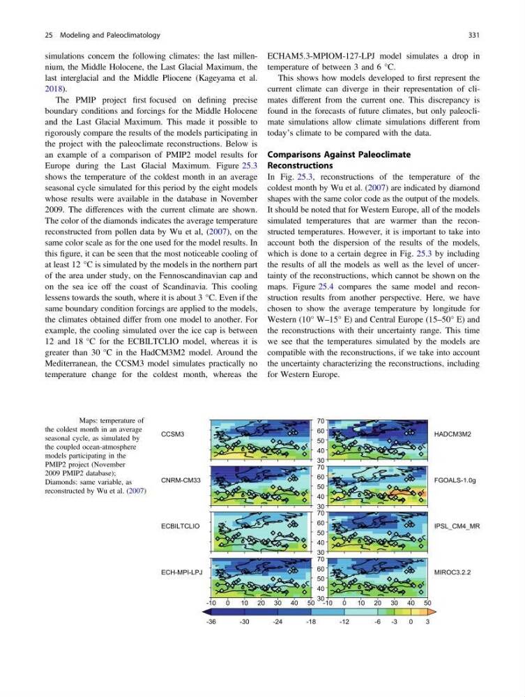
Europe during the Last Glacial Maximum. Figure 25.3
shows the temperature of the coldest month in an average
seasonal cycle simulated for this period by the eight models
whose results were available in the database in November
2009. The differences with the current climate are shown.
The color of the diamonds indicates the average temperature
reconstructed from pollen data by Wu et al, (2007), on the
same color scale as for the one used for the model results. In
this figure, it can be seen that the most noticeable cooling of
at least 12 °C is simulated by the models in the northern part
of the area under study, on the Fennoscandinavian cap and
on the sea ice off the coast of Scandinavia. This cooling
lessens towards the south, where it is about 3 °C. Even if the
same boundary condition forcings are applied to the models,
the climates obtained differ from one model to another. For
example, the cooling simulated over the ice cap is between
12 and 18 °C for the ECBILTCLIO model, whereas it is
greater than 30 °C in the HadCM3M2 model. Around the
Mediterranean, the CCSM3 model simulates practically no
temperature change for the coldest month, whereas the
ECHAM5.3-MPIOM-127-LPJ model simulates a drop in
temperature of between 3 and 6 °C.
This shows how models developed to first represent the
current climate can diverge in their representation of climates different from the current one. This discrepancy is
found in the forecasts of future climates, but only paleoclimate simulations allow climate simulations different from
today’s climate to be compared with the data.
Comparisons Against Paleoclimate
Reconstructions
In Fig. 25.3, reconstructions of the temperature of the
coldest month by Wu et al. (2007) are indicated by diamond
shapes with the same color code as the output of the models.
It should be noted that for Western Europe, all of the models
simulated temperatures that are warmer than the reconstructed temperatures. However, it is important to take into
account both the dispersion of the results of the models,
which is done to a certain degree in Fig. 25.3 by including
the results of all the models as well as the level of uncertainty of the reconstructions, which cannot be shown on the
maps. Figure 25.4 compares the same model and reconstruction results from another perspective. Here, we have
chosen to show the average temperature by longitude for
Western (10° W–15° E) and Central Europe (15–50° E) and
the reconstructions with their uncertainty range. This time
we see that the temperatures simulated by the models are
compatible with the reconstructions, if we take into account
the uncertainty characterizing the reconstructions, including
for Western Europe.
CCSM3
CNRM-CM33
0
-30
3
-24
-18
-12
-6
-36
-3
ECH-MPI-LPJ
0
4 0
10
50
20
-10
30
FGOALS-1.0g
70
40
50
60
30
HADCM3M2
70
40
50
60
30
MIROC3.2.2
0
4 0
10
50
20
-10
30
70
40
50
60
30
IPSL_CM4_MR
70
40
50
60
30
ECBILTCLIO
Fig. 25.3 Maps: temperature of
the coldest month in an average
seasonal cycle, as simulated by
the coupled ocean-atmosphere
models participating in the
PMIP2 project (November
2009 PMIP2 database);
Diamonds: same variable, as
reconstructed by Wu et al. (2007)
25 Modeling and Paleoclimatology
331
last interglacial and the Middle Pliocene (Kageyama et al.
2018).
The PMIP project first focused on defining precise
boundary conditions and forcings for the Middle Holocene
and the Last Glacial Maximum. This made it possible to
rigorously compare the results of the models participating in
the project with the paleoclimate reconstructions. Below is
an example of a comparison of PMIP2 model results for
Europe during the Last Glacial Maximum. Figure 25.3
shows the temperature of the coldest month in an average
seasonal cycle simulated for this period by the eight models
whose results were available in the database in November
2009. The differences with the current climate are shown.
The color of the diamonds indicates the average temperature
reconstructed from pollen data by Wu et al, (2007), on the
same color scale as for the one used for the model results. In
this figure, it can be seen that the most noticeable cooling of
at least 12 °C is simulated by the models in the northern part
of the area under study, on the Fennoscandinavian cap and
on the sea ice off the coast of Scandinavia. This cooling
lessens towards the south, where it is about 3 °C. Even if the
same boundary condition forcings are applied to the models,
the climates obtained differ from one model to another. For
example, the cooling simulated over the ice cap is between
12 and 18 °C for the ECBILTCLIO model, whereas it is
greater than 30 °C in the HadCM3M2 model. Around the
Mediterranean, the CCSM3 model simulates practically no
temperature change for the coldest month, whereas the
ECHAM5.3-MPIOM-127-LPJ model simulates a drop in
temperature of between 3 and 6 °C.
This shows how models developed to first represent the
current climate can diverge in their representation of climates different from the current one. This discrepancy is
found in the forecasts of future climates, but only paleoclimate simulations allow climate simulations different from
today’s climate to be compared with the data.
Comparisons Against Paleoclimate
Reconstructions
In Fig. 25.3, reconstructions of the temperature of the
coldest month by Wu et al. (2007) are indicated by diamond
shapes with the same color code as the output of the models.
It should be noted that for Western Europe, all of the models
simulated temperatures that are warmer than the reconstructed temperatures. However, it is important to take into
account both the dispersion of the results of the models,
which is done to a certain degree in Fig. 25.3 by including
the results of all the models as well as the level of uncertainty of the reconstructions, which cannot be shown on the
maps. Figure 25.4 compares the same model and reconstruction results from another perspective. Here, we have
chosen to show the average temperature by longitude for
Western (10° W–15° E) and Central Europe (15–50° E) and
the reconstructions with their uncertainty range. This time
we see that the temperatures simulated by the models are
compatible with the reconstructions, if we take into account
the uncertainty characterizing the reconstructions, including
for Western Europe.
CCSM3
CNRM-CM33
0
-30
3
-24
-18
-12
-6
-36
-3
ECH-MPI-LPJ
0
4 0
10
50
20
-10
30
FGOALS-1.0g
70
40
50
60
30
HADCM3M2
70
40
50
60
30
MIROC3.2.2
0
4 0
10
50
20
-10
30
70
40
50
60
30
IPSL_CM4_MR
70
40
50
60
30
ECBILTCLIO
Fig. 25.3 Maps: temperature of
the coldest month in an average
seasonal cycle, as simulated by
the coupled ocean-atmosphere
models participating in the
PMIP2 project (November
2009 PMIP2 database);
Diamonds: same variable, as
reconstructed by Wu et al. (2007)
25 Modeling and Paleoclimatology
331