

produces the land temperatures/precipitation values most
compatible with the reconstructed data. These are known
as sensitivity experiments to sea surface temperatures.
In the case discussed above, we examined several scenarios with different ocean surface temperatures to find out
which was most realistic for the period in question. More
generally, it is also instructive to analyze the signature or
influence of each forcing among several forcings and
changes in boundary conditions. To continue with the
example of the climate of the Last Glacial Maximum, if a
coupled atmosphere-ocean model is used, the forcings
applied to the model to obtain a simulation of the climate of
this period are:
1. the insolation;
2. the greenhouse gas concentration (CO 2 , CH 4 , N 2 O);
3. the altitude and extent of the ice caps and the change in
land-ocean distribution caused by changes in sea level.
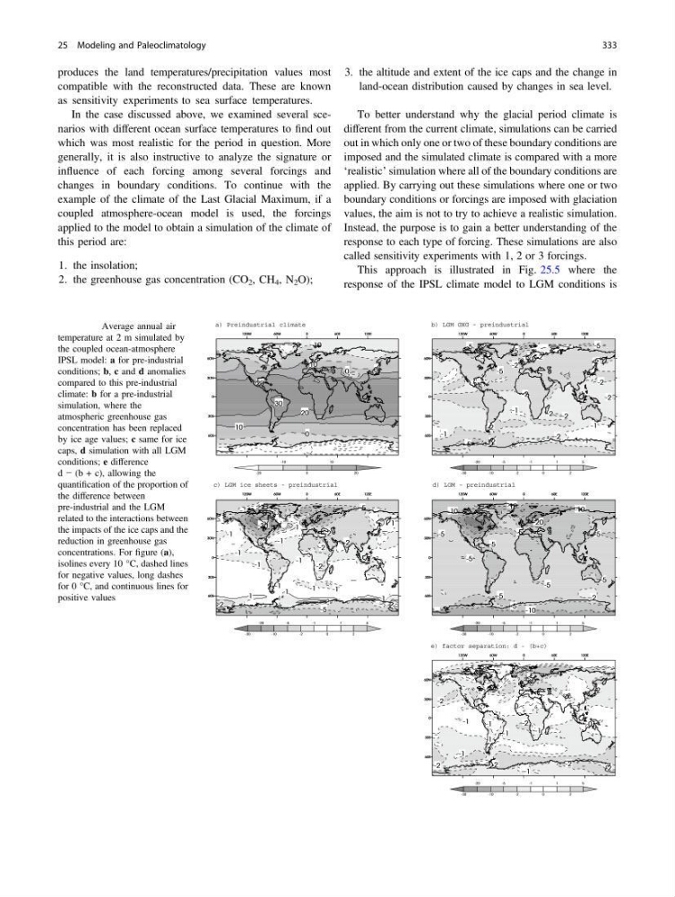
To better understand why the glacial period climate is
different from the current climate, simulations can be carried
out in which only one or two of these boundary conditions are
imposed and the simulated climate is compared with a more
‘realistic’ simulation where all of the boundary conditions are
applied. By carrying out these simulations where one or two
boundary conditions or forcings are imposed with glaciation
values, the aim is not to try to achieve a realistic simulation.
Instead, the purpose is to gain a better understanding of the
response to each type of forcing. These simulations are also
called sensitivity experiments with 1, 2 or 3 forcings.
This approach is illustrated in Fig. 25.5 where the
response of the IPSL climate model to LGM conditions is
Fig. 25.5 Average annual air
temperature at 2 m simulated by
the coupled ocean-atmosphere
IPSL model: a for pre-industrial
conditions; b, c and d anomalies
compared to this pre-industrial
climate: b for a pre-industrial
simulation, where the
atmospheric greenhouse gas
concentration has been replaced
by ice age values; c same for ice
caps, d simulation with all LGM
conditions; e difference
d − (b + c), allowing the
quantification of the proportion of
the difference between
pre-industrial and the LGM
related to the interactions between
the impacts of the ice caps and the
reduction in greenhouse gas
concentrations. For figure (a),
isolines every 10 °C, dashed lines
for negative values, long dashes
for 0 °C, and continuous lines for
positive values
25 Modeling and Paleoclimatology
333
compatible with the reconstructed data. These are known
as sensitivity experiments to sea surface temperatures.
In the case discussed above, we examined several scenarios with different ocean surface temperatures to find out
which was most realistic for the period in question. More
generally, it is also instructive to analyze the signature or
influence of each forcing among several forcings and
changes in boundary conditions. To continue with the
example of the climate of the Last Glacial Maximum, if a
coupled atmosphere-ocean model is used, the forcings
applied to the model to obtain a simulation of the climate of
this period are:
1. the insolation;
2. the greenhouse gas concentration (CO 2 , CH 4 , N 2 O);
3. the altitude and extent of the ice caps and the change in
land-ocean distribution caused by changes in sea level.
To better understand why the glacial period climate is
different from the current climate, simulations can be carried
out in which only one or two of these boundary conditions are
imposed and the simulated climate is compared with a more
‘realistic’ simulation where all of the boundary conditions are
applied. By carrying out these simulations where one or two
boundary conditions or forcings are imposed with glaciation
values, the aim is not to try to achieve a realistic simulation.
Instead, the purpose is to gain a better understanding of the
response to each type of forcing. These simulations are also
called sensitivity experiments with 1, 2 or 3 forcings.
This approach is illustrated in Fig. 25.5 where the
response of the IPSL climate model to LGM conditions is
Fig. 25.5 Average annual air
temperature at 2 m simulated by
the coupled ocean-atmosphere
IPSL model: a for pre-industrial
conditions; b, c and d anomalies
compared to this pre-industrial
climate: b for a pre-industrial
simulation, where the
atmospheric greenhouse gas
concentration has been replaced
by ice age values; c same for ice
caps, d simulation with all LGM
conditions; e difference
d − (b + c), allowing the
quantification of the proportion of
the difference between
pre-industrial and the LGM
related to the interactions between
the impacts of the ice caps and the
reduction in greenhouse gas
concentrations. For figure (a),
isolines every 10 °C, dashed lines
for negative values, long dashes
for 0 °C, and continuous lines for
positive values
25 Modeling and Paleoclimatology
333