

13 Theoretical Generalization of the Optical Chirality to Arbitrary Optical Media
345
1
2
E · ∂ t (∇ × P) = ∂ t
N −1
n=0
∂ t P n · (∇ × ∂ t P n ) + ω
2
n P n · (∇ × ×P n )
2ε 0 f n ω 2
p
−
N −1
n=0
ω
2
n ∂ t P n · (∇ × ×P n ) + ∂ t P n ·
∇ × ∂
2
t P n
2ε 0 f n ω 2
p
+
N −1
n=0
γ n ∂ t P n · (∇ × ∂ t P n )
2ε 0 f n ω 2
p
;
(13.65a)
1
2
H · ∂ t (∇ × M) = ∂ t
N −1
n=0
∂ t M n · (∇ × ∂ t M n ) + ˜
ω
2
n M n · (∇ × ×M n )
2 ˜
f n ˜
ω 2
n
−
N −1
n=0
˜
ω
2
n ∂ t M n · (∇ × ×M n ) + ∂ t M n ·
∇ × ∂
2
t M n
2 ˜
f n ˜
ω 2
n
+
N −1
n=0
˜
γ n ∂ t M n · (∇ × ∂ t M n )
˜
f n ˜
ω 2
n
.
(13.65b)
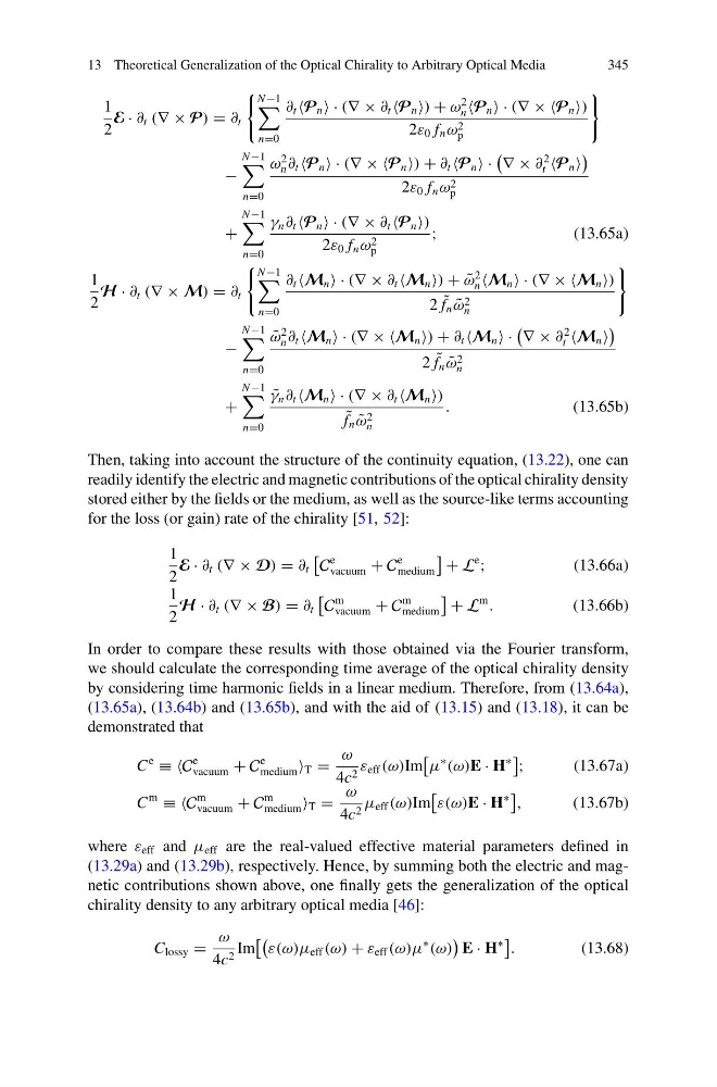
Then, taking into account the structure of the continuity equation, (13.22), one can
readily identify the electric and magnetic contributions of the optical chirality density
stored either by the fields or the medium, as well as the source-like terms accounting
for the loss (or gain) rate of the chirality [51, 52]:
1
2
E · ∂ t (∇ × D) = ∂ t
C
e
vacuum + C
e
medium
+ L
e
;
(13.66a)
1
2
H · ∂ t (∇ × B) = ∂ t
C
m
vacuum + C
m
medium
+ L
m
.
(13.66b)
In order to compare these results with those obtained via the Fourier transform,
we should calculate the corresponding time average of the optical chirality density
by considering time harmonic fields in a linear medium. Therefore, from (13.64a),
(13.65a), (13.64b) and (13.65b), and with the aid of (13.15) and (13.18), it can be
demonstrated that
C
e
≡ ≡C
e
vacuum + C
e
medium T =
ω
4c 2 ε eff (ω)Im
μ
∗
(ω)E · H
∗
;
(13.67a)
C
m
≡ ≡C
m
vacuum + C
m
medium T =
ω
4c 2 μ eff (ω)Im
ε(ω)E · H
∗
,
(13.67b)
where ε eff and μ eff are the real-valued effective material parameters defined in
(13.29a) and (13.29b), respectively. Hence, by summing both the electric and magnetic contributions shown above, one finally gets the generalization of the optical
chirality density to any arbitrary optical media [46]:
C lossy =
ω
4c 2 Im
ε(ω)μ eff (ω) + ε eff (ω)μ
∗
(ω)
E · H
∗
.
(13.68)
345
1
2
E · ∂ t (∇ × P) = ∂ t
N −1
n=0
∂ t P n · (∇ × ∂ t P n ) + ω
2
n P n · (∇ × ×P n )
2ε 0 f n ω 2
p
−
N −1
n=0
ω
2
n ∂ t P n · (∇ × ×P n ) + ∂ t P n ·
∇ × ∂
2
t P n
2ε 0 f n ω 2
p
+
N −1
n=0
γ n ∂ t P n · (∇ × ∂ t P n )
2ε 0 f n ω 2
p
;
(13.65a)
1
2
H · ∂ t (∇ × M) = ∂ t
N −1
n=0
∂ t M n · (∇ × ∂ t M n ) + ˜
ω
2
n M n · (∇ × ×M n )
2 ˜
f n ˜
ω 2
n
−
N −1
n=0
˜
ω
2
n ∂ t M n · (∇ × ×M n ) + ∂ t M n ·
∇ × ∂
2
t M n
2 ˜
f n ˜
ω 2
n
+
N −1
n=0
˜
γ n ∂ t M n · (∇ × ∂ t M n )
˜
f n ˜
ω 2
n
.
(13.65b)
Then, taking into account the structure of the continuity equation, (13.22), one can
readily identify the electric and magnetic contributions of the optical chirality density
stored either by the fields or the medium, as well as the source-like terms accounting
for the loss (or gain) rate of the chirality [51, 52]:
1
2
E · ∂ t (∇ × D) = ∂ t
C
e
vacuum + C
e
medium
+ L
e
;
(13.66a)
1
2
H · ∂ t (∇ × B) = ∂ t
C
m
vacuum + C
m
medium
+ L
m
.
(13.66b)
In order to compare these results with those obtained via the Fourier transform,
we should calculate the corresponding time average of the optical chirality density
by considering time harmonic fields in a linear medium. Therefore, from (13.64a),
(13.65a), (13.64b) and (13.65b), and with the aid of (13.15) and (13.18), it can be
demonstrated that
C
e
≡ ≡C
e
vacuum + C
e
medium T =
ω
4c 2 ε eff (ω)Im
μ
∗
(ω)E · H
∗
;
(13.67a)
C
m
≡ ≡C
m
vacuum + C
m
medium T =
ω
4c 2 μ eff (ω)Im
ε(ω)E · H
∗
,
(13.67b)
where ε eff and μ eff are the real-valued effective material parameters defined in
(13.29a) and (13.29b), respectively. Hence, by summing both the electric and magnetic contributions shown above, one finally gets the generalization of the optical
chirality density to any arbitrary optical media [46]:
C lossy =
ω
4c 2 Im
ε(ω)μ eff (ω) + ε eff (ω)μ
∗
(ω)
E · H
∗
.
(13.68)