

346
J. E. Vázquez-Lozano and A. Martínez
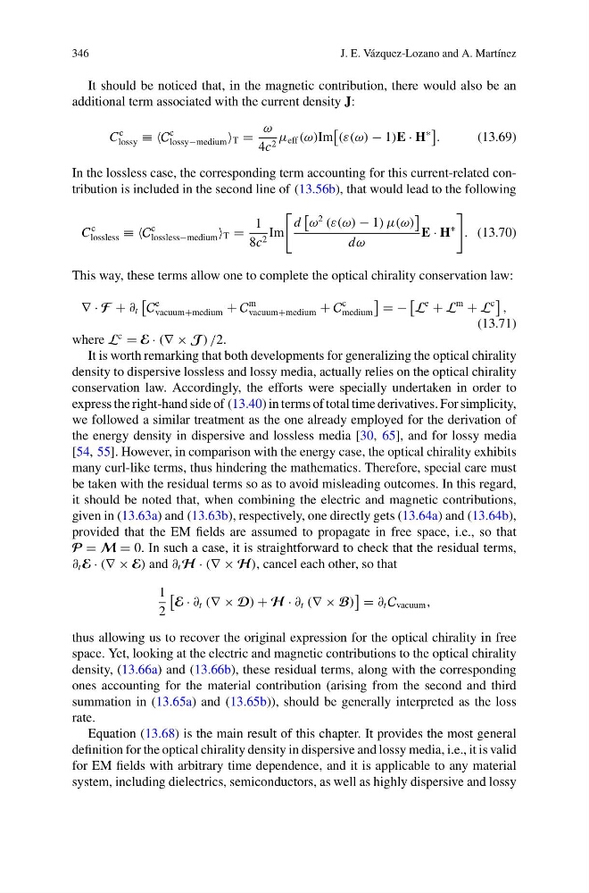
It should be noticed that, in the magnetic contribution, there would also be an
additional term associated with the current density J:
C
c
lossy ≡ ≡C
c
lossy−medium T =
ω
4c 2 μ eff (ω)Im
(ε(ω) − 1)E · H
∗
.
(13.69)
In the lossless case, the corresponding term accounting for this current-related contribution is included in the second line of (13.56b), that would lead to the following
C
c
lossless ≡ ≡C
c
lossless−medium T =
1
8c 2 Im
d
ω
2
(ε(ω) − 1) μ(ω)
dω
E · H
∗
. (13.70)
This way, these terms allow one to complete the optical chirality conservation law:
∇ · F + ∂ t
C
e
vacuum+medium + C
m
vacuum+medium + C
c
medium
= −
L
e
+ L
m
+ L
c
,
(13.71)
where L
c
= E · (∇ × J ) /2.
It is worth remarking that both developments for generalizing the optical chirality
density to dispersive lossless and lossy media, actually relies on the optical chirality
conservation law. Accordingly, the efforts were specially undertaken in order to
express the right-hand side of (13.40) in terms of total time derivatives. For simplicity,
we followed a similar treatment as the one already employed for the derivation of
the energy density in dispersive and lossless media [30, 65], and for lossy media
[54, 55]. However, in comparison with the energy case, the optical chirality exhibits
many curl-like terms, thus hindering the mathematics. Therefore, special care must
be taken with the residual terms so as to avoid misleading outcomes. In this regard,
it should be noted that, when combining the electric and magnetic contributions,
given in (13.63a) and (13.63b), respectively, one directly gets (13.64a) and (13.64b),
provided that the EM fields are assumed to propagate in free space, i.e., so that
P = M = 0. In such a case, it is straightforward to check that the residual terms,
∂ t E · (∇ × E) and ∂ t H · (∇ × H), cancel each other, so that
1
2
E · ∂ t (∇ × D) + H · ∂ t (∇ × B)
= ∂ t C vacuum ,
thus allowing us to recover the original expression for the optical chirality in free
space. Yet, looking at the electric and magnetic contributions to the optical chirality
density, (13.66a) and (13.66b), these residual terms, along with the corresponding
ones accounting for the material contribution (arising from the second and third
summation in (13.65a) and (13.65b)), should be generally interpreted as the loss
rate.
Equation (13.68) is the main result of this chapter. It provides the most general
definition for the optical chirality density in dispersive and lossy media, i.e., it is valid
for EM fields with arbitrary time dependence, and it is applicable to any material
system, including dielectrics, semiconductors, as well as highly dispersive and lossy
J. E. Vázquez-Lozano and A. Martínez
It should be noticed that, in the magnetic contribution, there would also be an
additional term associated with the current density J:
C
c
lossy ≡ ≡C
c
lossy−medium T =
ω
4c 2 μ eff (ω)Im
(ε(ω) − 1)E · H
∗
.
(13.69)
In the lossless case, the corresponding term accounting for this current-related contribution is included in the second line of (13.56b), that would lead to the following
C
c
lossless ≡ ≡C
c
lossless−medium T =
1
8c 2 Im
d
ω
2
(ε(ω) − 1) μ(ω)
dω
E · H
∗
. (13.70)
This way, these terms allow one to complete the optical chirality conservation law:
∇ · F + ∂ t
C
e
vacuum+medium + C
m
vacuum+medium + C
c
medium
= −
L
e
+ L
m
+ L
c
,
(13.71)
where L
c
= E · (∇ × J ) /2.
It is worth remarking that both developments for generalizing the optical chirality
density to dispersive lossless and lossy media, actually relies on the optical chirality
conservation law. Accordingly, the efforts were specially undertaken in order to
express the right-hand side of (13.40) in terms of total time derivatives. For simplicity,
we followed a similar treatment as the one already employed for the derivation of
the energy density in dispersive and lossless media [30, 65], and for lossy media
[54, 55]. However, in comparison with the energy case, the optical chirality exhibits
many curl-like terms, thus hindering the mathematics. Therefore, special care must
be taken with the residual terms so as to avoid misleading outcomes. In this regard,
it should be noted that, when combining the electric and magnetic contributions,
given in (13.63a) and (13.63b), respectively, one directly gets (13.64a) and (13.64b),
provided that the EM fields are assumed to propagate in free space, i.e., so that
P = M = 0. In such a case, it is straightforward to check that the residual terms,
∂ t E · (∇ × E) and ∂ t H · (∇ × H), cancel each other, so that
1
2
E · ∂ t (∇ × D) + H · ∂ t (∇ × B)
= ∂ t C vacuum ,
thus allowing us to recover the original expression for the optical chirality in free
space. Yet, looking at the electric and magnetic contributions to the optical chirality
density, (13.66a) and (13.66b), these residual terms, along with the corresponding
ones accounting for the material contribution (arising from the second and third
summation in (13.65a) and (13.65b)), should be generally interpreted as the loss
rate.
Equation (13.68) is the main result of this chapter. It provides the most general
definition for the optical chirality density in dispersive and lossy media, i.e., it is valid
for EM fields with arbitrary time dependence, and it is applicable to any material
system, including dielectrics, semiconductors, as well as highly dispersive and lossy