

334
J. E. Vázquez-Lozano and A. Martínez
∇ · S + ∂ t
W
e
+ W
m
= −
L
e
+ L
m
+ L
c
.
(13.27)
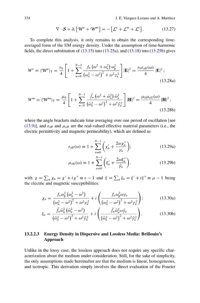
To complete this analysis, it only remains to obtain the corresponding timeaveraged form of the EM energy density. Under the assumption of time-harmonic
fields, the direct substitution of (13.15) into (13.25a), and (13.18) into (13.25b) gives
W
e
≡ ≡W
e
T =
ε 0
4
1 +
N −1
n=0
f n
ω
2
+ ω
2
n
ω
2
p
ω 2
n − ω 2
2 + ω 2 γ 2
n
|E|
2
=
ε 0 ε eff (ω)
4
|E|
2
;
(13.28a)
W
m
≡ ≡W
m
T =
μ 0
4
1 +
N −1
n=0
˜
f n
ω
2
+ ˜
ω
2
n
˜
ω
2
n
˜
ω 2
n − ω 2
2 + ω 2 ˜
γ 2
n
|H|
2
=
μ 0 μ eff (ω)
4
|H|
2
,
(13.28b)
where the angle brackets indicate time averaging over one period of oscillation [see
(13.9)], and ε eff and μ eff are the real-valued effective material parameters (i.e., the
electric permittivity and magnetic permeability), which are defined as
ε eff (ω) ≡ 1 +
N −1
n=0
χ
n +
2ωχ
n
γ n
;
(13.29a)
μ eff (ω) ≡ 1 +
N −1
n=0
ξ
n +
2ωξ
n
˜
γ n
,
(13.29b)
with χ =
n χ n = χ
+ iχ
≡ ε − 1 and ξ =
n ξ n = ξ
+ iξ
≡ μ − 1 being
the electric and magnetic susceptibilities:
χ n =
f n ω
2
p
ω
2
n − ω
2
ω 2
n − ω 2
2 + ω 2 γ 2
n
+ i
f n ω
2
p ωγ n
ω 2
n − ω 2
2 + ω 2 γ 2
n
;
(13.30a)
ξ n =
˜
f n ˜
ω
2
n
˜
ω
2
n − ω
2
˜
ω 2
n − ω 2
2 + ω 2 ˜
γ 2
n
+ i
˜
f n ˜
ω
2
n ω ˜
γ n
˜
ω 2
n − ω 2
2 + ω 2 ˜
γ 2
n
.
(13.30b)
13.2.2.3 Energy Density in Dispersive and Lossless Media: Brillouin’s
Approach
Unlike in the lossy case, the lossless approach does not require any specific characterization about the medium under consideration. Still, for the sake of simplicity,
the only assumptions made hereinafter are that the medium is linear, homogeneous,
and isotropic. This derivation simply involves the direct evaluation of the Fourier
J. E. Vázquez-Lozano and A. Martínez
∇ · S + ∂ t
W
e
+ W
m
= −
L
e
+ L
m
+ L
c
.
(13.27)
To complete this analysis, it only remains to obtain the corresponding timeaveraged form of the EM energy density. Under the assumption of time-harmonic
fields, the direct substitution of (13.15) into (13.25a), and (13.18) into (13.25b) gives
W
e
≡ ≡W
e
T =
ε 0
4
1 +
N −1
n=0
f n
ω
2
+ ω
2
n
ω
2
p
ω 2
n − ω 2
2 + ω 2 γ 2
n
|E|
2
=
ε 0 ε eff (ω)
4
|E|
2
;
(13.28a)
W
m
≡ ≡W
m
T =
μ 0
4
1 +
N −1
n=0
˜
f n
ω
2
+ ˜
ω
2
n
˜
ω
2
n
˜
ω 2
n − ω 2
2 + ω 2 ˜
γ 2
n
|H|
2
=
μ 0 μ eff (ω)
4
|H|
2
,
(13.28b)
where the angle brackets indicate time averaging over one period of oscillation [see
(13.9)], and ε eff and μ eff are the real-valued effective material parameters (i.e., the
electric permittivity and magnetic permeability), which are defined as
ε eff (ω) ≡ 1 +
N −1
n=0
χ
n +
2ωχ
n
γ n
;
(13.29a)
μ eff (ω) ≡ 1 +
N −1
n=0
ξ
n +
2ωξ
n
˜
γ n
,
(13.29b)
with χ =
n χ n = χ
+ iχ
≡ ε − 1 and ξ =
n ξ n = ξ
+ iξ
≡ μ − 1 being
the electric and magnetic susceptibilities:
χ n =
f n ω
2
p
ω
2
n − ω
2
ω 2
n − ω 2
2 + ω 2 γ 2
n
+ i
f n ω
2
p ωγ n
ω 2
n − ω 2
2 + ω 2 γ 2
n
;
(13.30a)
ξ n =
˜
f n ˜
ω
2
n
˜
ω
2
n − ω
2
˜
ω 2
n − ω 2
2 + ω 2 ˜
γ 2
n
+ i
˜
f n ˜
ω
2
n ω ˜
γ n
˜
ω 2
n − ω 2
2 + ω 2 ˜
γ 2
n
.
(13.30b)
13.2.2.3 Energy Density in Dispersive and Lossless Media: Brillouin’s
Approach
Unlike in the lossy case, the lossless approach does not require any specific characterization about the medium under consideration. Still, for the sake of simplicity,
the only assumptions made hereinafter are that the medium is linear, homogeneous,
and isotropic. This derivation simply involves the direct evaluation of the Fourier