

332
J. E. Vázquez-Lozano and A. Martínez
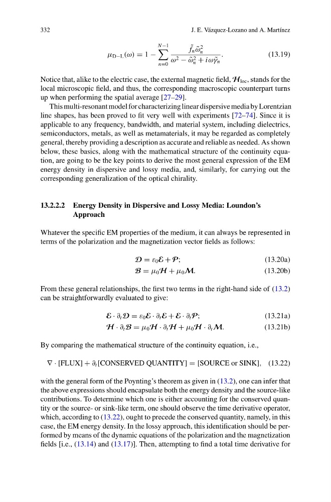
μ D−L (ω) = 1 −
N −1
n=0
˜
f n ˜
ω
2
n
ω 2 − ˜
ω 2
n + iω ˜
γ n
.
(13.19)
Notice that, alike to the electric case, the external magnetic field, H loc , stands for the
local microscopic field, and thus, the corresponding macroscopic counterpart turns
up when performing the spatial average [27–29].
This multi-resonant model for characterizing linear dispersive media by Lorentzian
line shapes, has been proved to fit very well with experiments [72–74]. Since it is
applicable to any frequency, bandwidth, and material system, including dielectrics,
semiconductors, metals, as well as metamaterials, it may be regarded as completely
general, thereby providing a description as accurate and reliable as needed. As shown
below, these basics, along with the mathematical structure of the continuity equation, are going to be the key points to derive the most general expression of the EM
energy density in dispersive and lossy media, and, similarly, for carrying out the
corresponding generalization of the optical chirality.
13.2.2.2 Energy Density in Dispersive and Lossy Media: Loundon’s
Approach
Whatever the specific EM properties of the medium, it can always be represented in
terms of the polarization and the magnetization vector fields as follows:
D = ε 0 E + P;
(13.20a)
B = μ 0 H + μ 0 M.
(13.20b)
From these general relationships, the first two terms in the right-hand side of (13.2)
can be straightforwardly evaluated to give:
E · ∂ t D = ε 0 E · ∂ t E + E · ∂ t P;
(13.21a)
H · ∂ t B = μ 0 H · ∂ t H + μ 0 H · ∂ t M.
(13.21b)
By comparing the mathematical structure of the continuity equation, i.e.,
∇ · [FLUX] + ∂ t [CONSERVED QUANTITY] = [SOURCE or SINK], (13.22)
with the general form of the Poynting’s theorem as given in (13.2), one can infer that
the above expressions should encapsulate both the energy density and the source-like
contributions. To determine which one is either accounting for the conserved quantity or the source- or sink-like term, one should observe the time derivative operator,
which, according to (13.22), ought to precede the conserved quantity, namely, in this
case, the EM energy density. In the lossy approach, this identification should be performed by means of the dynamic equations of the polarization and the magnetization
fields [i.e., (13.14) and (13.17)]. Then, attempting to find a total time derivative for
J. E. Vázquez-Lozano and A. Martínez
μ D−L (ω) = 1 −
N −1
n=0
˜
f n ˜
ω
2
n
ω 2 − ˜
ω 2
n + iω ˜
γ n
.
(13.19)
Notice that, alike to the electric case, the external magnetic field, H loc , stands for the
local microscopic field, and thus, the corresponding macroscopic counterpart turns
up when performing the spatial average [27–29].
This multi-resonant model for characterizing linear dispersive media by Lorentzian
line shapes, has been proved to fit very well with experiments [72–74]. Since it is
applicable to any frequency, bandwidth, and material system, including dielectrics,
semiconductors, metals, as well as metamaterials, it may be regarded as completely
general, thereby providing a description as accurate and reliable as needed. As shown
below, these basics, along with the mathematical structure of the continuity equation, are going to be the key points to derive the most general expression of the EM
energy density in dispersive and lossy media, and, similarly, for carrying out the
corresponding generalization of the optical chirality.
13.2.2.2 Energy Density in Dispersive and Lossy Media: Loundon’s
Approach
Whatever the specific EM properties of the medium, it can always be represented in
terms of the polarization and the magnetization vector fields as follows:
D = ε 0 E + P;
(13.20a)
B = μ 0 H + μ 0 M.
(13.20b)
From these general relationships, the first two terms in the right-hand side of (13.2)
can be straightforwardly evaluated to give:
E · ∂ t D = ε 0 E · ∂ t E + E · ∂ t P;
(13.21a)
H · ∂ t B = μ 0 H · ∂ t H + μ 0 H · ∂ t M.
(13.21b)
By comparing the mathematical structure of the continuity equation, i.e.,
∇ · [FLUX] + ∂ t [CONSERVED QUANTITY] = [SOURCE or SINK], (13.22)
with the general form of the Poynting’s theorem as given in (13.2), one can infer that
the above expressions should encapsulate both the energy density and the source-like
contributions. To determine which one is either accounting for the conserved quantity or the source- or sink-like term, one should observe the time derivative operator,
which, according to (13.22), ought to precede the conserved quantity, namely, in this
case, the EM energy density. In the lossy approach, this identification should be performed by means of the dynamic equations of the polarization and the magnetization
fields [i.e., (13.14) and (13.17)]. Then, attempting to find a total time derivative for