

306
F. Vanderveken et al.
given by (12.14) and (12.52), exist for the coupled set of equations. These solutions
correspond to magnetoelastic waves. However, it is important to keep in mind that
for large dynamic components, a system of nonlinear differential equations has to be
solved, including nonlinear magnetoelastic interaction effects.
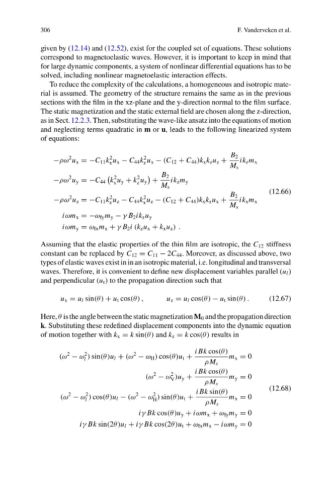
To reduce the complexity of the calculations, a homogeneous and isotropic material is assumed. The geometry of the structure remains the same as in the previous
sections with the film in the xz-plane and the y-direction normal to the film surface.
The static magnetization and the static external field are chosen along the z-direction,
as in Sect. 12.2.3. Then, substituting the wave-like ansatz into the equations of motion
and neglecting terms quadratic in m or u, leads to the following linearized system
of equations:
−ρω
2 u x = −C 11 k
2
x u x − C 44 k
2
z u x − (C 12 + C 44 )k x k z u z +
B 2
M s
ik z m x
−ρω
2 u y = −C 44
k
2
x u y + k
2
z u y
+
B 2
M s
ik z m y
−ρω
2 u z = −C 11 k
2
z u z − C 44 k
2
x u z − (C 12 + C 44 )k x k z u x +
B 2
M s
ik x m x
iωm x = −ω fy m y − γ B 2 ik z u y
iωm y = ω fx m x + γ B 2 i (k z u x + k x u z ) .
(12.66)
Assuming that the elastic properties of the thin film are isotropic, the C 12 stiffness
constant can be replaced by C 12 = C 11 − 2C 44 . Moreover, as discussed above, two
types of elastic waves exist in in an isotropic material, i.e. longitudinal and transversal
waves. Therefore, it is convenient to define new displacement variables parallel (u l )
and perpendicular (u t ) to the propagation direction such that
u x = u l sin(θ ) + u t cos(θ ) ,
u z = u l cos(θ ) − u t sin(θ ) .
(12.67)
Here, θ is the angle between the static magnetization M 0 and the propagation direction
k. Substituting these redefined displacement components into the dynamic equation
of motion together with k x = k sin(θ ) and k z = k cos(θ ) results in
(ω
2
− ω
2
l ) sin(θ )u l + (ω
2
− ω H ) cos(θ )u t +
i Bk cos(θ )
ρ M s
m x = 0
(ω
2
− ω
2
V )u y +
i Bk cos(θ )
ρ M s
m y = 0
(ω
2
− ω
2
l ) cos(θ )u l − (ω
2
− ω
2
H ) sin(θ )u t +
i Bk sin(θ )
ρ M s
m x = 0
iγ Bk cos(θ )u y + iωm x + ω fy m y = 0
iγ Bk sin(2θ)u l + iγ Bk cos(2θ)u t + ω fx m x − iωm y = 0
(12.68)
F. Vanderveken et al.
given by (12.14) and (12.52), exist for the coupled set of equations. These solutions
correspond to magnetoelastic waves. However, it is important to keep in mind that
for large dynamic components, a system of nonlinear differential equations has to be
solved, including nonlinear magnetoelastic interaction effects.
To reduce the complexity of the calculations, a homogeneous and isotropic material is assumed. The geometry of the structure remains the same as in the previous
sections with the film in the xz-plane and the y-direction normal to the film surface.
The static magnetization and the static external field are chosen along the z-direction,
as in Sect. 12.2.3. Then, substituting the wave-like ansatz into the equations of motion
and neglecting terms quadratic in m or u, leads to the following linearized system
of equations:
−ρω
2 u x = −C 11 k
2
x u x − C 44 k
2
z u x − (C 12 + C 44 )k x k z u z +
B 2
M s
ik z m x
−ρω
2 u y = −C 44
k
2
x u y + k
2
z u y
+
B 2
M s
ik z m y
−ρω
2 u z = −C 11 k
2
z u z − C 44 k
2
x u z − (C 12 + C 44 )k x k z u x +
B 2
M s
ik x m x
iωm x = −ω fy m y − γ B 2 ik z u y
iωm y = ω fx m x + γ B 2 i (k z u x + k x u z ) .
(12.66)
Assuming that the elastic properties of the thin film are isotropic, the C 12 stiffness
constant can be replaced by C 12 = C 11 − 2C 44 . Moreover, as discussed above, two
types of elastic waves exist in in an isotropic material, i.e. longitudinal and transversal
waves. Therefore, it is convenient to define new displacement variables parallel (u l )
and perpendicular (u t ) to the propagation direction such that
u x = u l sin(θ ) + u t cos(θ ) ,
u z = u l cos(θ ) − u t sin(θ ) .
(12.67)
Here, θ is the angle between the static magnetization M 0 and the propagation direction
k. Substituting these redefined displacement components into the dynamic equation
of motion together with k x = k sin(θ ) and k z = k cos(θ ) results in
(ω
2
− ω
2
l ) sin(θ )u l + (ω
2
− ω H ) cos(θ )u t +
i Bk cos(θ )
ρ M s
m x = 0
(ω
2
− ω
2
V )u y +
i Bk cos(θ )
ρ M s
m y = 0
(ω
2
− ω
2
l ) cos(θ )u l − (ω
2
− ω
2
H ) sin(θ )u t +
i Bk sin(θ )
ρ M s
m x = 0
iγ Bk cos(θ )u y + iωm x + ω fy m y = 0
iγ Bk sin(2θ)u l + iγ Bk cos(2θ)u t + ω fx m x − iωm y = 0
(12.68)