

292
F. Vanderveken et al.
12.2.2 Spin Waves in the Bulk Ferromagnets
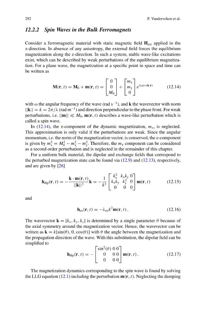
Consider a ferromagnetic material with static magnetic field H ext applied in the
z-direction. In absence of any anisotropy, the external field forces the equilibrium
magnetization along the z-direction. In such a system, stable wave-like excitations
exist, which can be described by weak perturbations of the equilibrium magnetization. For a plane wave, the magnetization at a specific point in space and time can
be written as
M(r, t) = M 0 + m(r, t) =
⎡
⎣
0
0
M 0
⎤
⎦ +
⎡
⎣
m x
m y
0
⎤
⎦ e
i(ωt+k·r)
(12.14)
with ω the angular frequency of the wave (rad s
−1 ), and k the wavevector with norm
||k|| = k = 2π/λ (rad m
−1 ) and direction perpendicular to the phase front. For weak
perturbations, i.e. ||m|| | M 0 , m(r, t) describes a wave-like perturbation which is
called a spin wave.
In (12.14), the z-component of the dynamic magnetization, m z , is neglected.
This approximation is only valid if the perturbations are weak. Since the angular
momentum, i.e. the norm of the magnetization vector, is conserved, the z-component
is given by m
2
z = M
2
0 − m
2
x − m
2
y . Therefore, the m z component can be considered
as a second order perturbation and is neglected in the remainder of this chapter.
For a uniform bulk material, the dipolar and exchange fields that correspond to
the perturbed magnetization state can be found via (12.9) and (12.13), respectively,
and are given by [26]
h dip (r, t) = −
k · m(r, t)
||k|| 2 k = −
1
k 2
⎡
⎣
k
2
x k x k y 0
k x k y k
2
y 0
0
0 0
⎤
⎦ m(r, t)
(12.15)
and
h ex (r, t) = −λ ex k
2 m(r, t) .
(12.16)
The wavevector k = [k x , k y , k z ] is determined by a single parameter θ because of
the axial symmetry around the magnetization vector. Hence, the wavevector can be
written as k = k[sin(θ ), 0, cos(θ )] with θ the angle between the magnetization and
the propagation direction of the wave. With this substitution, the dipolar field can be
simplified to
h dip (r, t) = −
⎡
⎣
sin
2
(θ ) 0 0
0 0 0
0 0 0
⎤
⎦ m(r, t) .
(12.17)
The magnetization dynamics corresponding to the spin wave is found by solving
the LLG equation (12.1) including the perturbation m(r, t). Neglecting the damping
F. Vanderveken et al.
12.2.2 Spin Waves in the Bulk Ferromagnets
Consider a ferromagnetic material with static magnetic field H ext applied in the
z-direction. In absence of any anisotropy, the external field forces the equilibrium
magnetization along the z-direction. In such a system, stable wave-like excitations
exist, which can be described by weak perturbations of the equilibrium magnetization. For a plane wave, the magnetization at a specific point in space and time can
be written as
M(r, t) = M 0 + m(r, t) =
⎡
⎣
0
0
M 0
⎤
⎦ +
⎡
⎣
m x
m y
0
⎤
⎦ e
i(ωt+k·r)
(12.14)
with ω the angular frequency of the wave (rad s
−1 ), and k the wavevector with norm
||k|| = k = 2π/λ (rad m
−1 ) and direction perpendicular to the phase front. For weak
perturbations, i.e. ||m|| | M 0 , m(r, t) describes a wave-like perturbation which is
called a spin wave.
In (12.14), the z-component of the dynamic magnetization, m z , is neglected.
This approximation is only valid if the perturbations are weak. Since the angular
momentum, i.e. the norm of the magnetization vector, is conserved, the z-component
is given by m
2
z = M
2
0 − m
2
x − m
2
y . Therefore, the m z component can be considered
as a second order perturbation and is neglected in the remainder of this chapter.
For a uniform bulk material, the dipolar and exchange fields that correspond to
the perturbed magnetization state can be found via (12.9) and (12.13), respectively,
and are given by [26]
h dip (r, t) = −
k · m(r, t)
||k|| 2 k = −
1
k 2
⎡
⎣
k
2
x k x k y 0
k x k y k
2
y 0
0
0 0
⎤
⎦ m(r, t)
(12.15)
and
h ex (r, t) = −λ ex k
2 m(r, t) .
(12.16)
The wavevector k = [k x , k y , k z ] is determined by a single parameter θ because of
the axial symmetry around the magnetization vector. Hence, the wavevector can be
written as k = k[sin(θ ), 0, cos(θ )] with θ the angle between the magnetization and
the propagation direction of the wave. With this substitution, the dipolar field can be
simplified to
h dip (r, t) = −
⎡
⎣
sin
2
(θ ) 0 0
0 0 0
0 0 0
⎤
⎦ m(r, t) .
(12.17)
The magnetization dynamics corresponding to the spin wave is found by solving
the LLG equation (12.1) including the perturbation m(r, t). Neglecting the damping