

11 Floquet Theory and Ultrafast Control of Magnetism
269
11.2.2 Discretized Fourier Transformation and Matrix Form
of Schrødinger Equation
Bloch theorem for solid crystals leads to their electron band structure [33, 34].
Following a similar manner, I here show that a generalized eigenvalue problem
appears by applying Floquet theorem to periodically-driven systems. It tells us a
basic physical picture of the driven systems.
The periodicity of ˆ
H (t + T ) = ˆ
H (t) and (t + T ) = (t) indicate that ˆ
H (t)
and (t) can both be Fourier-transformed along time direction in a discretized way.
We define their Fourier transforms as
ˆ
H (t) =
m∈Z
e
−imωt ˆ
H m ,
,(t) =
m∈Z
e
−imωt
m .
(11.9)
The inverse transformation is given by
ˆ
H m = T
−1
T
0
dt e
imωt ˆ
H (t),
, m = T
−1
T
0
dt e
imωt
(t).
(11.10)
Substituting these and (11.2) into the Schrødinger equation, we obtain the following
generalized eigenvalue problem for { ˆ
H m } and { m }:
n∈Z
( ˆ
H m+n − mωδ m,n )) n = m .
(11.11)
Therefore, with the set of Hamiltonians { ˆ
H m }, we can compute the wave functions
{ m } and the corresponding quasi energy (i.e., eigenvalue) in principle. Since the
real number is introduced in the form of e
−iT , its physical relevant range is ristricted
in the “Brillouin” zone −
π
T
= −
ω
2
≤ <
ω
2
=
π
T
like crystal momentum k in
solids. Due to this periodicity, is called quasi energy. We emphasize that (11.11)
does not explicitly depend on time t, and in that sense, it may be called a static
eigenvalue equation.
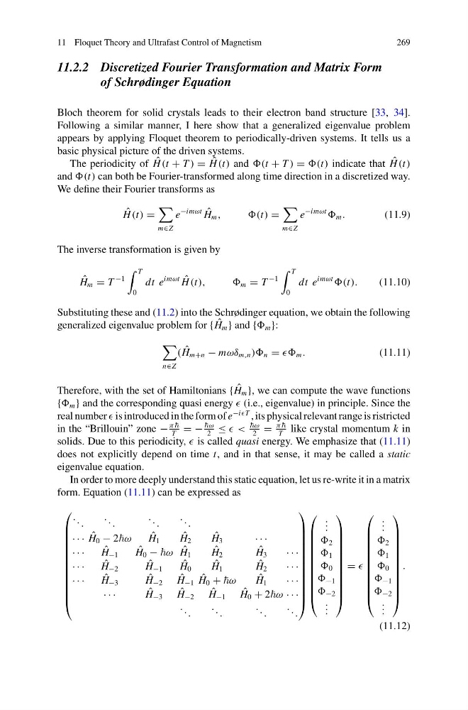
In order to more deeply understand this static equation, let us re-write it in a matrix
form. Equation (11.11) can be expressed as
⎛
⎜
⎜
⎜
⎜
⎜
⎜
⎜
⎜
⎜
⎜
⎜
⎝
. . .
. . .
. . .
. . .
· · · ˆ
H 0 − 2ω
ˆ
H 1
ˆ
H 2
ˆ
H 3
· · ·
· · ·
ˆ
H −1
ˆ
H 0 − ω ˆ
H 1
ˆ
H 2
ˆ
H 3
· · ·
· · ·
ˆ
H −2
ˆ
H −1
ˆ
H 0
ˆ
H 1
ˆ
H 2
· · ·
· · ·
ˆ
H −3
ˆ
H −2
ˆ
H −1 ˆ
H 0 + ω
ˆ
H 1
· · ·
· · ·
ˆ
H −3
ˆ
H −2
ˆ
H −1
ˆ
H 0 + 2ω · · ·
. . .
. . .
. . .
. . .
⎞
⎟
⎟
⎟
⎟
⎟
⎟
⎟
⎟
⎟
⎟
⎟
⎠
⎛
⎜
⎜
⎜
⎜
⎜
⎜
⎜
⎜
⎜
⎜
⎝
. . .
2
1
0
−1
−2
. . .
⎞
⎟
⎟
⎟
⎟
⎟
⎟
⎟
⎟
⎟
⎟
⎠
=
⎛
⎜
⎜
⎜
⎜
⎜
⎜
⎜
⎜
⎜
⎜
⎝
. . .
2
1
0
−1
−2
. . .
⎞
⎟
⎟
⎟
⎟
⎟
⎟
⎟
⎟
⎟
⎟
⎠
.
(11.12)
269
11.2.2 Discretized Fourier Transformation and Matrix Form
of Schrødinger Equation
Bloch theorem for solid crystals leads to their electron band structure [33, 34].
Following a similar manner, I here show that a generalized eigenvalue problem
appears by applying Floquet theorem to periodically-driven systems. It tells us a
basic physical picture of the driven systems.
The periodicity of ˆ
H (t + T ) = ˆ
H (t) and (t + T ) = (t) indicate that ˆ
H (t)
and (t) can both be Fourier-transformed along time direction in a discretized way.
We define their Fourier transforms as
ˆ
H (t) =
m∈Z
e
−imωt ˆ
H m ,
,(t) =
m∈Z
e
−imωt
m .
(11.9)
The inverse transformation is given by
ˆ
H m = T
−1
T
0
dt e
imωt ˆ
H (t),
, m = T
−1
T
0
dt e
imωt
(t).
(11.10)
Substituting these and (11.2) into the Schrødinger equation, we obtain the following
generalized eigenvalue problem for { ˆ
H m } and { m }:
n∈Z
( ˆ
H m+n − mωδ m,n )) n = m .
(11.11)
Therefore, with the set of Hamiltonians { ˆ
H m }, we can compute the wave functions
{ m } and the corresponding quasi energy (i.e., eigenvalue) in principle. Since the
real number is introduced in the form of e
−iT , its physical relevant range is ristricted
in the “Brillouin” zone −
π
T
= −
ω
2
≤ <
ω
2
=
π
T
like crystal momentum k in
solids. Due to this periodicity, is called quasi energy. We emphasize that (11.11)
does not explicitly depend on time t, and in that sense, it may be called a static
eigenvalue equation.
In order to more deeply understand this static equation, let us re-write it in a matrix
form. Equation (11.11) can be expressed as
⎛
⎜
⎜
⎜
⎜
⎜
⎜
⎜
⎜
⎜
⎜
⎜
⎝
. . .
. . .
. . .
. . .
· · · ˆ
H 0 − 2ω
ˆ
H 1
ˆ
H 2
ˆ
H 3
· · ·
· · ·
ˆ
H −1
ˆ
H 0 − ω ˆ
H 1
ˆ
H 2
ˆ
H 3
· · ·
· · ·
ˆ
H −2
ˆ
H −1
ˆ
H 0
ˆ
H 1
ˆ
H 2
· · ·
· · ·
ˆ
H −3
ˆ
H −2
ˆ
H −1 ˆ
H 0 + ω
ˆ
H 1
· · ·
· · ·
ˆ
H −3
ˆ
H −2
ˆ
H −1
ˆ
H 0 + 2ω · · ·
. . .
. . .
. . .
. . .
⎞
⎟
⎟
⎟
⎟
⎟
⎟
⎟
⎟
⎟
⎟
⎟
⎠
⎛
⎜
⎜
⎜
⎜
⎜
⎜
⎜
⎜
⎜
⎜
⎝
. . .
2
1
0
−1
−2
. . .
⎞
⎟
⎟
⎟
⎟
⎟
⎟
⎟
⎟
⎟
⎟
⎠
=
⎛
⎜
⎜
⎜
⎜
⎜
⎜
⎜
⎜
⎜
⎜
⎝
. . .
2
1
0
−1
−2
. . .
⎞
⎟
⎟
⎟
⎟
⎟
⎟
⎟
⎟
⎟
⎟
⎠
.
(11.12)