

9 Symmetry Approach to Chiral Optomagnonics in Antiferromagnetic Insulators
231
space, a i =
k exp(i k · r i )a k and b i =
k exp(i k · r i )b k , we can rewrite (9.78) in
the following form
ˆ
H =
k
A k
a
†
k a k + b
†
−k b −k
+ B k a k b −k + B
∗
k a
†
k b
†
−k
,
(9.80)
where parameters A k and B k include microscopic details. For example, in the case
when the exchange interactions are limited by the nearest neighboring sites so
that J i j = J
i j = J 1 , we obtain A k = 2K S + Z J 1 S and B k = J 1 S
δ exp(−i k · δ),
where δ connects a site on the A sublattice with its Z nearest neighboring sites on
the B sublattice.
9.4.3.1 Magnon Spin Currents: Quantum Version
The expression for a magnon spin current can be derived following the same steps as
in Sect. 9.4.1. Considering the equation of motion for the z component of the local
spin density, n(r i ) = b
†
i b i − a
†
i a i , we find the total magnon spin current
ˆ
J s =
k
∂ A k
∂ k
a
†
k a k + b
†
−k b −k
+
∂ B k
∂ k
a k b −k +
∂ B
∗
k
∂ k
a
†
k b
†
−k
.
(9.81)
This expression can be conveniently written in the matrix form
ˆ
J s =
k
χ
†
k
∂H k
∂ k
χ k ,
(9.82)
where we introduced χ k =
a k
b
†
−k
and H k =
A k B
∗
k
B k A k
. Note that in this representation, χ k does not satisfy boson communication relations; instead one has
[χ k , χ
†
k
] = σ z δ k,k
, which should be kept in mind.
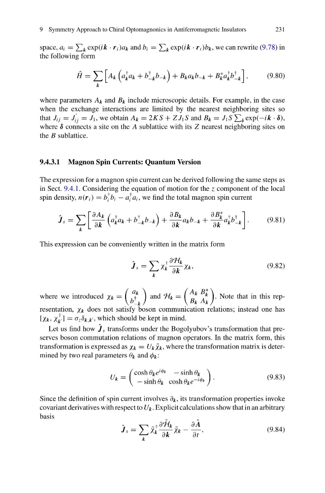
Let us find how ˆ
J s transforms under the Bogolyubov’s transformation that preserves boson commutation relations of magnon operators. In the matrix form, this
transformation is expressed as χ k = U k ˜
χ k , where the transformation matrix is determined by two real parameters θ k and φ k :
U k =
cosh θ k e
iφ k − sinh θ k
− sinh θ k cosh θ k e
−iφ k
.
(9.83)
Since the definition of spin current involves ∂ k , its transformation properties invoke
covariant derivatives with respect to U k . Explicit calculations show that in an arbitrary
basis
ˆ
J s =
k
˜
χ
†
k
∂ ˜
H k
∂ k
˜
χ k −
∂ ˆ
A
∂t
,
(9.84)
231
space, a i =
k exp(i k · r i )a k and b i =
k exp(i k · r i )b k , we can rewrite (9.78) in
the following form
ˆ
H =
k
A k
a
†
k a k + b
†
−k b −k
+ B k a k b −k + B
∗
k a
†
k b
†
−k
,
(9.80)
where parameters A k and B k include microscopic details. For example, in the case
when the exchange interactions are limited by the nearest neighboring sites so
that J i j = J
i j = J 1 , we obtain A k = 2K S + Z J 1 S and B k = J 1 S
δ exp(−i k · δ),
where δ connects a site on the A sublattice with its Z nearest neighboring sites on
the B sublattice.
9.4.3.1 Magnon Spin Currents: Quantum Version
The expression for a magnon spin current can be derived following the same steps as
in Sect. 9.4.1. Considering the equation of motion for the z component of the local
spin density, n(r i ) = b
†
i b i − a
†
i a i , we find the total magnon spin current
ˆ
J s =
k
∂ A k
∂ k
a
†
k a k + b
†
−k b −k
+
∂ B k
∂ k
a k b −k +
∂ B
∗
k
∂ k
a
†
k b
†
−k
.
(9.81)
This expression can be conveniently written in the matrix form
ˆ
J s =
k
χ
†
k
∂H k
∂ k
χ k ,
(9.82)
where we introduced χ k =
a k
b
†
−k
and H k =
A k B
∗
k
B k A k
. Note that in this representation, χ k does not satisfy boson communication relations; instead one has
[χ k , χ
†
k
] = σ z δ k,k
, which should be kept in mind.
Let us find how ˆ
J s transforms under the Bogolyubov’s transformation that preserves boson commutation relations of magnon operators. In the matrix form, this
transformation is expressed as χ k = U k ˜
χ k , where the transformation matrix is determined by two real parameters θ k and φ k :
U k =
cosh θ k e
iφ k − sinh θ k
− sinh θ k cosh θ k e
−iφ k
.
(9.83)
Since the definition of spin current involves ∂ k , its transformation properties invoke
covariant derivatives with respect to U k . Explicit calculations show that in an arbitrary
basis
ˆ
J s =
k
˜
χ
†
k
∂ ˜
H k
∂ k
˜
χ k −
∂ ˆ
A
∂t
,
(9.84)