

8 Microwave-Driven Dynamics of Magnetic Skyrmions …
199
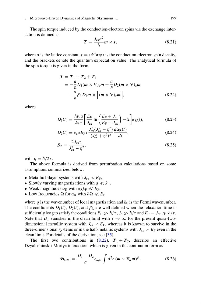
The spin torque induced by the conduction-electron spins via the exchange interaction is defined as
T =
J ex a
2
m × s,
(8.21)
where a is the lattice constant, s = =ψ
†
σ ψ is the conduction-electron spin density,
and the brackets denote the quantum expectation value. The analytical formula of
the spin torque is given in the form,
T = T 1 + T 2 + T 3
= −
a
D 1 (m × ∇) z m +
a
D 2 (m × ∇) z m
−
a
β R D 2 m ×
(m × ∇) z m
,
(8.22)
where
D 1 (t) =
ν e a
2πτ
E F
J ex
ln
E F + J ex
E F − J ex
− 2
α R (t),
(8.23)
D 2 (t) = ν e a E F τ
J
2
ex (J
2
ex − η
2
)
(J 2
ex + η 2 ) 2
dα R (t)
dt
,
(8.24)
β R =
2J ex η
J 2
ex − η 2 ,
(8.25)
with η = /2τ .
The above formula is derived from perturbation calculations based on some
assumptions summarized below:
• Metallic bilayer systems with J ex < E F ,
• Slowly varying magnetizations with q k F ,
• Weak magnitudes α R with α R k F E F ,
• Low frequencies for α R with E F ,
where q is the wavenumber of local magnetization and k F is the Fermi wavenumber.
The coefficients D 1 (t), D 2 (t), and β R are well defined when the relaxation time is
sufficiently long to satisfy the conditions E F /τ , J e /τ and E F − J ex /τ .
Note that D 1 vanishes in the clean limit with τ → ∞ for the present quasi-twodimensional metallic system with J ex < E F , whereas it is known to survive in the
three-dimensional systems or in the half-metallic systems with J ex > E F even in the
clean limit. For details of the derivation, see [35].
The first two contributions in (8.22), T 1 + T 2 , describe an effective
Dzyaloshinskii-Moriya interaction, which is given in the continuum form as
H DMI =
D 1 − D 2
a
αβz
d
2 r (m × ∇ α m)
β
.
(8.26)
199
The spin torque induced by the conduction-electron spins via the exchange interaction is defined as
T =
J ex a
2
m × s,
(8.21)
where a is the lattice constant, s = =ψ
†
σ ψ is the conduction-electron spin density,
and the brackets denote the quantum expectation value. The analytical formula of
the spin torque is given in the form,
T = T 1 + T 2 + T 3
= −
a
D 1 (m × ∇) z m +
a
D 2 (m × ∇) z m
−
a
β R D 2 m ×
(m × ∇) z m
,
(8.22)
where
D 1 (t) =
ν e a
2πτ
E F
J ex
ln
E F + J ex
E F − J ex
− 2
α R (t),
(8.23)
D 2 (t) = ν e a E F τ
J
2
ex (J
2
ex − η
2
)
(J 2
ex + η 2 ) 2
dα R (t)
dt
,
(8.24)
β R =
2J ex η
J 2
ex − η 2 ,
(8.25)
with η = /2τ .
The above formula is derived from perturbation calculations based on some
assumptions summarized below:
• Metallic bilayer systems with J ex < E F ,
• Slowly varying magnetizations with q k F ,
• Weak magnitudes α R with α R k F E F ,
• Low frequencies for α R with E F ,
where q is the wavenumber of local magnetization and k F is the Fermi wavenumber.
The coefficients D 1 (t), D 2 (t), and β R are well defined when the relaxation time is
sufficiently long to satisfy the conditions E F /τ , J e /τ and E F − J ex /τ .
Note that D 1 vanishes in the clean limit with τ → ∞ for the present quasi-twodimensional metallic system with J ex < E F , whereas it is known to survive in the
three-dimensional systems or in the half-metallic systems with J ex > E F even in the
clean limit. For details of the derivation, see [35].
The first two contributions in (8.22), T 1 + T 2 , describe an effective
Dzyaloshinskii-Moriya interaction, which is given in the continuum form as
H DMI =
D 1 − D 2
a
αβz
d
2 r (m × ∇ α m)
β
.
(8.26)