

7 Current-Induced Dynamics of Chiral Magnetic Structures
163
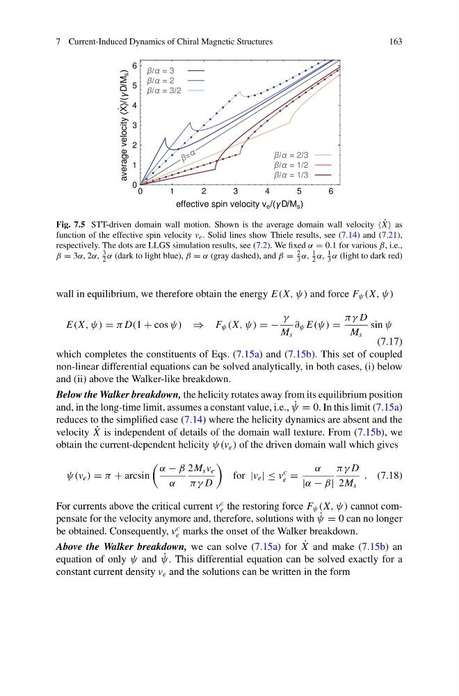
Fig. 7.5 STT-driven domain wall motion. Shown is the average domain wall velocity ˙
X as
function of the effective spin velocity v e . Solid lines show Thiele results, see (7.14) and (7.21),
respectively. The dots are LLGS simulation results, see (7.2). We fixed α = 0.1 for various β, i.e.,
β = 3α, 2α,
3
2 α (dark to light blue), β = α (gray dashed), and β =
2
3 α,
1
2 α,
1
3 α (light to dark red)
wall in equilibrium, we therefore obtain the energy E(X, ψ) and force F ψ (X, ψ)
E(X, ψ) = π D(1 + cos ψ) ⇒ F ψ (X, ψ) = −
γ
M s
∂ ψ E(ψ) =
πγ D
M s
sin ψ
(7.17)
which completes the constituents of Eqs. (7.15a) and (7.15b). This set of coupled
non-linear differential equations can be solved analytically, in both cases, (i) below
and (ii) above the Walker-like breakdown.
Below the Walker breakdown, the helicity rotates away from its equilibrium position
and, in the long-time limit, assumes a constant value, i.e., ˙
ψ = 0. In this limit (7.15a)
reduces to the simplified case (7.14) where the helicity dynamics are absent and the
velocity ˙
X is independent of details of the domain wall texture. From (7.15b), we
obtain the current-dependent helicity ψ(v e ) of the driven domain wall which gives
ψ(v e ) = π + arcsin
α − β
α
2M s v e
πγ D
for |v e | ≤ v
c
e =
α
|α − β|
πγ D
2M s
. (7.18)
For currents above the critical current v
c
e the restoring force F ψ (X, ψ) cannot compensate for the velocity anymore and, therefore, solutions with ˙
ψ = 0 can no longer
be obtained. Consequently, v
c
e marks the onset of the Walker breakdown.
Above the Walker breakdown, we can solve (7.15a) for ˙
X and make (7.15b) an
equation of only ψ and ˙
ψ. This differential equation can be solved exactly for a
constant current density v e and the solutions can be written in the form
163
Fig. 7.5 STT-driven domain wall motion. Shown is the average domain wall velocity ˙
X as
function of the effective spin velocity v e . Solid lines show Thiele results, see (7.14) and (7.21),
respectively. The dots are LLGS simulation results, see (7.2). We fixed α = 0.1 for various β, i.e.,
β = 3α, 2α,
3
2 α (dark to light blue), β = α (gray dashed), and β =
2
3 α,
1
2 α,
1
3 α (light to dark red)
wall in equilibrium, we therefore obtain the energy E(X, ψ) and force F ψ (X, ψ)
E(X, ψ) = π D(1 + cos ψ) ⇒ F ψ (X, ψ) = −
γ
M s
∂ ψ E(ψ) =
πγ D
M s
sin ψ
(7.17)
which completes the constituents of Eqs. (7.15a) and (7.15b). This set of coupled
non-linear differential equations can be solved analytically, in both cases, (i) below
and (ii) above the Walker-like breakdown.
Below the Walker breakdown, the helicity rotates away from its equilibrium position
and, in the long-time limit, assumes a constant value, i.e., ˙
ψ = 0. In this limit (7.15a)
reduces to the simplified case (7.14) where the helicity dynamics are absent and the
velocity ˙
X is independent of details of the domain wall texture. From (7.15b), we
obtain the current-dependent helicity ψ(v e ) of the driven domain wall which gives
ψ(v e ) = π + arcsin
α − β
α
2M s v e
πγ D
for |v e | ≤ v
c
e =
α
|α − β|
πγ D
2M s
. (7.18)
For currents above the critical current v
c
e the restoring force F ψ (X, ψ) cannot compensate for the velocity anymore and, therefore, solutions with ˙
ψ = 0 can no longer
be obtained. Consequently, v
c
e marks the onset of the Walker breakdown.
Above the Walker breakdown, we can solve (7.15a) for ˙
X and make (7.15b) an
equation of only ψ and ˙
ψ. This differential equation can be solved exactly for a
constant current density v e and the solutions can be written in the form