

18 A Plausible Description of Continuum …
351
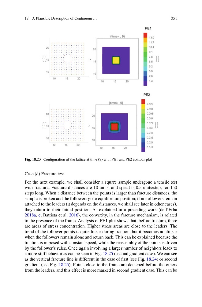
Fig. 18.23 Configuration of the lattice at time (9) with PE1 and PE2 contour plot
Case (d) Fracture test
For the next example, we shall consider a square sample undergone a tensile test
with fracture. Fracture distances are 10 units, and speed is 0.5 units/step, for 150
steps long. When a distance between the points is larger than fracture distances, the
sample is broken and the followers go to equilibrium position; if no followers remain
attached to the leaders (it depends on the distances, we shall see later in other cases),
they return to their initial position. As explained in a preceding work (dell’Erba
2018a, c; Battista et al. 2016), the convexity, in the fracture mechanism, is related
to the presence of the frame. Analysis of PE1 plot shows that, before fracture, there
are areas of stress concentration. Higher stress areas are close to the leaders. The
trend of the follower points is quite linear during traction, but it becomes nonlinear
when the followers remain alone and return back. This can be explained because the
traction is imposed with constant speed, while the reassembly of the points is driven
by the follower’s rules. Once again involving a larger number of neighbors leads to
a more stiff behavior as can be seen in Fig. 18.25 (second gradient case). We can see
as the vertical fracture line is different in the case of first (see Fig. 18.24) or second
gradient (see Fig. 18.25). Points close to the frame are detached before the others
from the leaders, and this effect is more marked in second gradient case. This can be
351
Fig. 18.23 Configuration of the lattice at time (9) with PE1 and PE2 contour plot
Case (d) Fracture test
For the next example, we shall consider a square sample undergone a tensile test
with fracture. Fracture distances are 10 units, and speed is 0.5 units/step, for 150
steps long. When a distance between the points is larger than fracture distances, the
sample is broken and the followers go to equilibrium position; if no followers remain
attached to the leaders (it depends on the distances, we shall see later in other cases),
they return to their initial position. As explained in a preceding work (dell’Erba
2018a, c; Battista et al. 2016), the convexity, in the fracture mechanism, is related
to the presence of the frame. Analysis of PE1 plot shows that, before fracture, there
are areas of stress concentration. Higher stress areas are close to the leaders. The
trend of the follower points is quite linear during traction, but it becomes nonlinear
when the followers remain alone and return back. This can be explained because the
traction is imposed with constant speed, while the reassembly of the points is driven
by the follower’s rules. Once again involving a larger number of neighbors leads to
a more stiff behavior as can be seen in Fig. 18.25 (second gradient case). We can see
as the vertical fracture line is different in the case of first (see Fig. 18.24) or second
gradient (see Fig. 18.25). Points close to the frame are detached before the others
from the leaders, and this effect is more marked in second gradient case. This can be