

352
R. dell’Erba
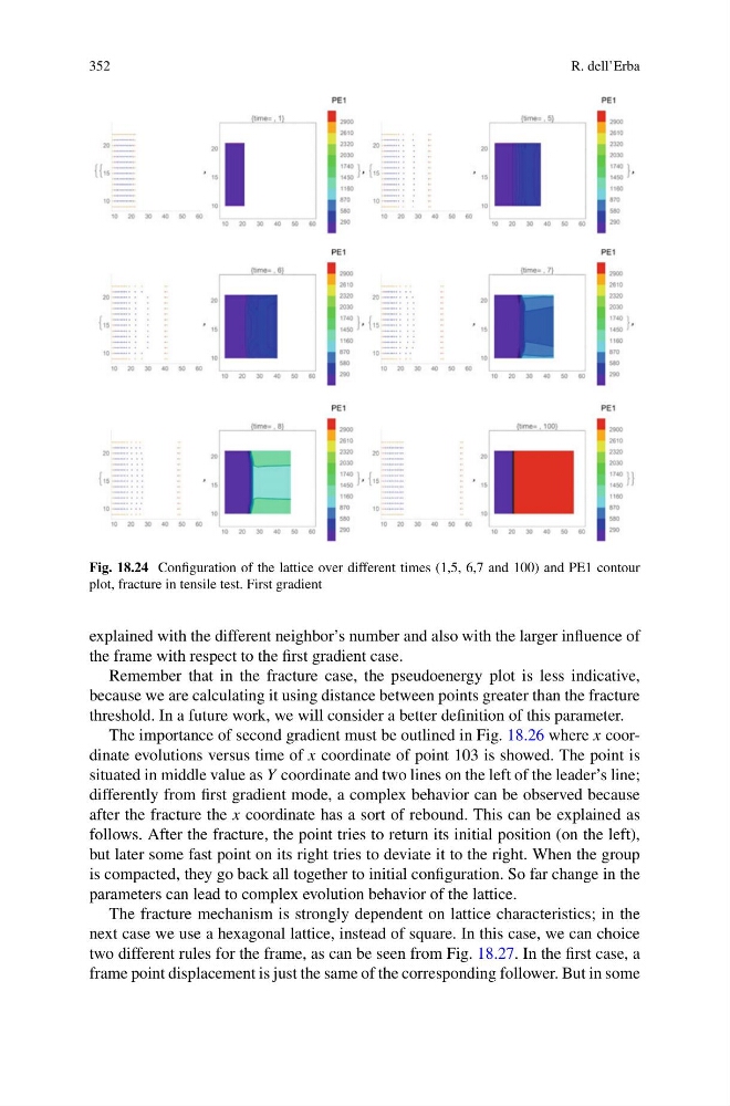
Fig. 18.24 Configuration of the lattice over different times (1,5, 6,7 and 100) and PE1 contour
plot, fracture in tensile test. First gradient
explained with the different neighbor’s number and also with the larger influence of
the frame with respect to the first gradient case.
Remember that in the fracture case, the pseudoenergy plot is less indicative,
because we are calculating it using distance between points greater than the fracture
threshold. In a future work, we will consider a better definition of this parameter.
The importance of second gradient must be outlined in Fig. 18.26 where x coordinate evolutions versus time of x coordinate of point 103 is showed. The point is
situated in middle value as Y coordinate and two lines on the left of the leader’s line;
differently from first gradient mode, a complex behavior can be observed because
after the fracture the x coordinate has a sort of rebound. This can be explained as
follows. After the fracture, the point tries to return its initial position (on the left),
but later some fast point on its right tries to deviate it to the right. When the group
is compacted, they go back all together to initial configuration. So far change in the
parameters can lead to complex evolution behavior of the lattice.
The fracture mechanism is strongly dependent on lattice characteristics; in the
next case we use a hexagonal lattice, instead of square. In this case, we can choice
two different rules for the frame, as can be seen from Fig. 18.27. In the first case, a
frame point displacement is just the same of the corresponding follower. But in some
R. dell’Erba
Fig. 18.24 Configuration of the lattice over different times (1,5, 6,7 and 100) and PE1 contour
plot, fracture in tensile test. First gradient
explained with the different neighbor’s number and also with the larger influence of
the frame with respect to the first gradient case.
Remember that in the fracture case, the pseudoenergy plot is less indicative,
because we are calculating it using distance between points greater than the fracture
threshold. In a future work, we will consider a better definition of this parameter.
The importance of second gradient must be outlined in Fig. 18.26 where x coordinate evolutions versus time of x coordinate of point 103 is showed. The point is
situated in middle value as Y coordinate and two lines on the left of the leader’s line;
differently from first gradient mode, a complex behavior can be observed because
after the fracture the x coordinate has a sort of rebound. This can be explained as
follows. After the fracture, the point tries to return its initial position (on the left),
but later some fast point on its right tries to deviate it to the right. When the group
is compacted, they go back all together to initial configuration. So far change in the
parameters can lead to complex evolution behavior of the lattice.
The fracture mechanism is strongly dependent on lattice characteristics; in the
next case we use a hexagonal lattice, instead of square. In this case, we can choice
two different rules for the frame, as can be seen from Fig. 18.27. In the first case, a
frame point displacement is just the same of the corresponding follower. But in some