

18 A Plausible Description of Continuum …
337
Leader
Frame
Follower
Neighbours 1st
Neighbours 2nd
2° gradient case
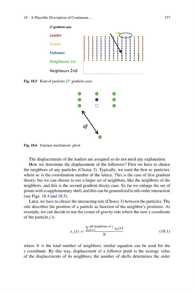
Fig. 18.5 Kind of particles (2° gradient case)
df
Fig. 18.6 Fracture mechanism: ghost
The displacements of the leaders are assigned so do not need any explanation.
How we determine the displacement of the followers? First we have to choice
the neighbors of any particles (Choice 2). Typically, we used the first nc particles,
where nc is the coordination number of the lattice. This is the case of first gradient
theory; but we can choose to use a larger set of neighbors, like the neighbors of the
neighbors, and this is the second gradient theory case. So far we enlarge the set of
points with a supplementary shell, and this can be generalized to nth-order interaction
(see Figs. 18.4 and 18.5).
Later, we have to choice the interacting rule (Choice 3) between the particles. The
rule describes the position of a particle as function of the neighbor’s positions. As
example, we can decide to use the center of gravity rule where the new x coordinate
of the particle j is
x j (t) =
all neighbours of j
k=1
x k (t)
N
(18.1)
where N is the total number of neighbors; similar equation can be used for the
y coordinate. By this way, displacement of a follower point is the average value
of the displacements of its neighbors; the number of shells determines the order
337
Leader
Frame
Follower
Neighbours 1st
Neighbours 2nd
2° gradient case
Fig. 18.5 Kind of particles (2° gradient case)
df
Fig. 18.6 Fracture mechanism: ghost
The displacements of the leaders are assigned so do not need any explanation.
How we determine the displacement of the followers? First we have to choice
the neighbors of any particles (Choice 2). Typically, we used the first nc particles,
where nc is the coordination number of the lattice. This is the case of first gradient
theory; but we can choose to use a larger set of neighbors, like the neighbors of the
neighbors, and this is the second gradient theory case. So far we enlarge the set of
points with a supplementary shell, and this can be generalized to nth-order interaction
(see Figs. 18.4 and 18.5).
Later, we have to choice the interacting rule (Choice 3) between the particles. The
rule describes the position of a particle as function of the neighbor’s positions. As
example, we can decide to use the center of gravity rule where the new x coordinate
of the particle j is
x j (t) =
all neighbours of j
k=1
x k (t)
N
(18.1)
where N is the total number of neighbors; similar equation can be used for the
y coordinate. By this way, displacement of a follower point is the average value
of the displacements of its neighbors; the number of shells determines the order