

338
R. dell’Erba
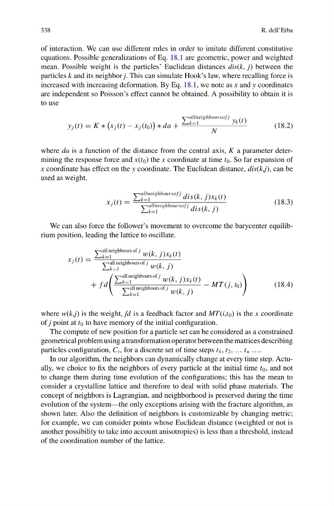
of interaction. We can use different rules in order to imitate different constitutive
equations. Possible generalizations of Eq. 18.1 are geometric, power and weighted
mean. Possible weight is the particles’ Euclidean distances dis(k, j) between the
particles k and its neighbor j. This can simulate Hook’s law, where recalling force is
increased with increasing deformation. By Eq. 18.1, we note as x and y coordinates
are independent so Poisson’s effect cannot be obtained. A possibility to obtain it is
to use
y j (t) = K ∗
x j (t) − x j (t 0 )
∗ da +
allneighbourso f j
k=1
y k (t)
N
(18.2)
where da is a function of the distance from the central axis, K a parameter determining the response force and x(t 0 ) the x coordinate at time t 0 . So far expansion of
x coordinate has effect on the y coordinate. The Euclidean distance, dis(k,j), can be
used as weight.
x j (t) =
allneighbourso f j
k=1
dis(k, j)x k (t)
allneighbourso f j
k=1
dis(k, j)
(18.3)
We can also force the follower’s movement to overcome the barycenter equilibrium position, leading the lattice to oscillate.
x j (t) =
all neighbours of j
k=1
w(k, j)x k (t)
all neighbours of j
k=1
w(k, j)
+ f d
all neighbours of j
k=1
w(k, j)x k (t)
all neighbours of j
k=1
w(k, j)
− MT ( j, t 0 )
(18.4)
where w(k,j) is the weight, fd is a feedback factor and MT (i,t 0 ) is the x coordinate
of j point at t 0 to have memory of the initial configuration.
The compute of new position for a particle set can be considered as a constrained
geometrical problem using a transformation operator between the matrices describing
particles configuration, C t , for a discrete set of time steps t 1 , t 2 , … t n ….
In our algorithm, the neighbors can dynamically change at every time step. Actually, we choice to fix the neighbors of every particle at the initial time t 0 , and not
to change them during time evolution of the configurations; this has the mean to
consider a crystalline lattice and therefore to deal with solid phase materials. The
concept of neighbors is Lagrangian, and neighborhood is preserved during the time
evolution of the system—the only exceptions arising with the fracture algorithm, as
shown later. Also the definition of neighbors is customizable by changing metric;
for example, we can consider points whose Euclidean distance (weighted or not is
another possibility to take into account anisotropies) is less than a threshold, instead
of the coordination number of the lattice.
R. dell’Erba
of interaction. We can use different rules in order to imitate different constitutive
equations. Possible generalizations of Eq. 18.1 are geometric, power and weighted
mean. Possible weight is the particles’ Euclidean distances dis(k, j) between the
particles k and its neighbor j. This can simulate Hook’s law, where recalling force is
increased with increasing deformation. By Eq. 18.1, we note as x and y coordinates
are independent so Poisson’s effect cannot be obtained. A possibility to obtain it is
to use
y j (t) = K ∗
x j (t) − x j (t 0 )
∗ da +
allneighbourso f j
k=1
y k (t)
N
(18.2)
where da is a function of the distance from the central axis, K a parameter determining the response force and x(t 0 ) the x coordinate at time t 0 . So far expansion of
x coordinate has effect on the y coordinate. The Euclidean distance, dis(k,j), can be
used as weight.
x j (t) =
allneighbourso f j
k=1
dis(k, j)x k (t)
allneighbourso f j
k=1
dis(k, j)
(18.3)
We can also force the follower’s movement to overcome the barycenter equilibrium position, leading the lattice to oscillate.
x j (t) =
all neighbours of j
k=1
w(k, j)x k (t)
all neighbours of j
k=1
w(k, j)
+ f d
all neighbours of j
k=1
w(k, j)x k (t)
all neighbours of j
k=1
w(k, j)
− MT ( j, t 0 )
(18.4)
where w(k,j) is the weight, fd is a feedback factor and MT (i,t 0 ) is the x coordinate
of j point at t 0 to have memory of the initial configuration.
The compute of new position for a particle set can be considered as a constrained
geometrical problem using a transformation operator between the matrices describing
particles configuration, C t , for a discrete set of time steps t 1 , t 2 , … t n ….
In our algorithm, the neighbors can dynamically change at every time step. Actually, we choice to fix the neighbors of every particle at the initial time t 0 , and not
to change them during time evolution of the configurations; this has the mean to
consider a crystalline lattice and therefore to deal with solid phase materials. The
concept of neighbors is Lagrangian, and neighborhood is preserved during the time
evolution of the system—the only exceptions arising with the fracture algorithm, as
shown later. Also the definition of neighbors is customizable by changing metric;
for example, we can consider points whose Euclidean distance (weighted or not is
another possibility to take into account anisotropies) is less than a threshold, instead
of the coordination number of the lattice.