

320
M. R. Karamooz-Ravari et al.
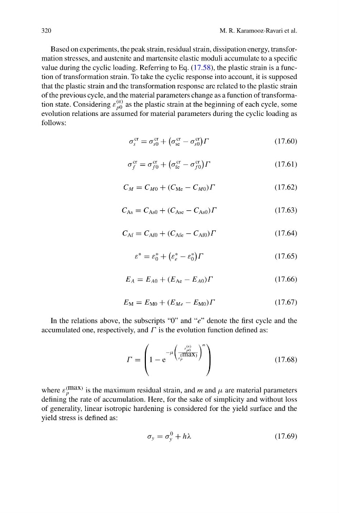
Based on experiments, the peak strain, residual strain, dissipation energy, transformation stresses, and austenite and martensite elastic moduli accumulate to a specific
value during the cyclic loading. Referring to Eq. (17.58), the plastic strain is a function of transformation strain. To take the cyclic response into account, it is supposed
that the plastic strain and the transformation response are related to the plastic strain
of the previous cycle, and the material parameters change as a function of transformation state. Considering ε
(n)
p0 as the plastic strain at the beginning of each cycle, some
evolution relations are assumed for material parameters during the cyclic loading as
follows:
σ
cr
s = σ
cr
s0 +
σ
cr
se − σ
cr
s0
Γ
(17.60)
σ
cr
f = σ
cr
f 0 +
σ
cr
fe − σ
cr
f 0
Γ
(17.61)
C M = C M0 + (C Me − C M0 )Γ
(17.62)
C As = C As0 + (C Ase − C As0 )Γ
(17.63)
C Af = C Af0 + (C Afe − C Af0 )Γ
(17.64)
ε
∗
= ε
∗
0 +
ε
∗
e − ε
∗
0
Γ
(17.65)
E A = E A0 + (E Ae − E A0 )Γ
(17.66)
E M = E M0 + (E Me − E M0 )Γ
(17.67)
In the relations above, the subscripts “0” and “e” denote the first cycle and the
accumulated one, respectively, and Γ is the evolution function defined as:
Γ =
⎛
⎜
⎝1 − e
−μ
ε
(n)
p0
ε
(max)
p
m ⎞
⎟
⎠
(17.68)
where ε
(max)
p
is the maximum residual strain, and m and μ are material parameters
defining the rate of accumulation. Here, for the sake of simplicity and without loss
of generality, linear isotropic hardening is considered for the yield surface and the
yield stress is defined as:
σ y = σ
0
y + hλ
(17.69)
M. R. Karamooz-Ravari et al.
Based on experiments, the peak strain, residual strain, dissipation energy, transformation stresses, and austenite and martensite elastic moduli accumulate to a specific
value during the cyclic loading. Referring to Eq. (17.58), the plastic strain is a function of transformation strain. To take the cyclic response into account, it is supposed
that the plastic strain and the transformation response are related to the plastic strain
of the previous cycle, and the material parameters change as a function of transformation state. Considering ε
(n)
p0 as the plastic strain at the beginning of each cycle, some
evolution relations are assumed for material parameters during the cyclic loading as
follows:
σ
cr
s = σ
cr
s0 +
σ
cr
se − σ
cr
s0
Γ
(17.60)
σ
cr
f = σ
cr
f 0 +
σ
cr
fe − σ
cr
f 0
Γ
(17.61)
C M = C M0 + (C Me − C M0 )Γ
(17.62)
C As = C As0 + (C Ase − C As0 )Γ
(17.63)
C Af = C Af0 + (C Afe − C Af0 )Γ
(17.64)
ε
∗
= ε
∗
0 +
ε
∗
e − ε
∗
0
Γ
(17.65)
E A = E A0 + (E Ae − E A0 )Γ
(17.66)
E M = E M0 + (E Me − E M0 )Γ
(17.67)
In the relations above, the subscripts “0” and “e” denote the first cycle and the
accumulated one, respectively, and Γ is the evolution function defined as:
Γ =
⎛
⎜
⎝1 − e
−μ
ε
(n)
p0
ε
(max)
p
m ⎞
⎟
⎠
(17.68)
where ε
(max)
p
is the maximum residual strain, and m and μ are material parameters
defining the rate of accumulation. Here, for the sake of simplicity and without loss
of generality, linear isotropic hardening is considered for the yield surface and the
yield stress is defined as:
σ y = σ
0
y + hλ
(17.69)