

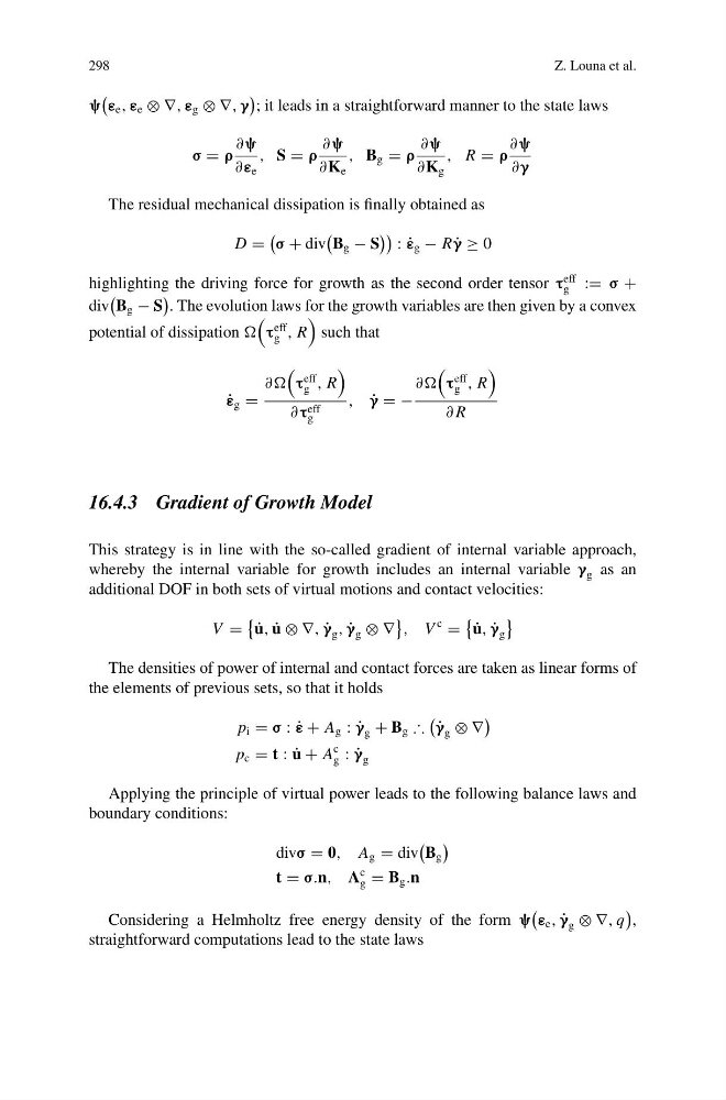
298
Z. Louna et al.
ψ
ε e , ε e ⊗ ∇, ε g ⊗ ∇, γ
; it leads in a straightforward manner to the state laws
σ = ρ
∂ψ
∂ε e
, S = ρ
∂ψ
∂K e
, B g = ρ
∂ψ
∂K g
, R = ρ
∂ψ
∂γ
The residual mechanical dissipation is finally obtained as
D =
σ + div
B g − S
: ˙
ε g − R ˙
γ ≥ 0
highlighting the driving force for growth as the second order tensor τ
eff
g := σ +
div
B g − S
. The evolution laws for the growth variables are then given by a convex
potential of dissipation
τ
eff
g , R
such that
˙
ε g =
∂∂
τ
eff
g , R
∂τ eff
g
, ˙
γ = −
∂∂
τ
eff
g , R
∂ R
16.4.3 Gradient of Growth Model
This strategy is in line with the so-called gradient of internal variable approach,
whereby the internal variable for growth includes an internal variable γ g as an
additional DOF in both sets of virtual motions and contact velocities:
V =
˙
u, ˙
u ⊗ ∇, ˙
γ g , ˙
γ g ⊗ ∇
, V
c
=
˙
u, ˙
γ g
The densities of power of internal and contact forces are taken as linear forms of
the elements of previous sets, so that it holds
p i = σ : ˙
ε + A g : ˙
γ g + B g ∴
˙
γ g ⊗ ∇
p c = t : ˙
u + A
c
g : ˙
γ g
Applying the principle of virtual power leads to the following balance laws and
boundary conditions:
divσ = 0, A g = div
B g
t = σ.n, A
c
g = B g .n
Considering a Helmholtz free energy density of the form ψ
ε e , ˙
γ g ⊗ ∇, q
,
straightforward computations lead to the state laws
Z. Louna et al.
ψ
ε e , ε e ⊗ ∇, ε g ⊗ ∇, γ
; it leads in a straightforward manner to the state laws
σ = ρ
∂ψ
∂ε e
, S = ρ
∂ψ
∂K e
, B g = ρ
∂ψ
∂K g
, R = ρ
∂ψ
∂γ
The residual mechanical dissipation is finally obtained as
D =
σ + div
B g − S
: ˙
ε g − R ˙
γ ≥ 0
highlighting the driving force for growth as the second order tensor τ
eff
g := σ +
div
B g − S
. The evolution laws for the growth variables are then given by a convex
potential of dissipation
τ
eff
g , R
such that
˙
ε g =
∂∂
τ
eff
g , R
∂τ eff
g
, ˙
γ = −
∂∂
τ
eff
g , R
∂ R
16.4.3 Gradient of Growth Model
This strategy is in line with the so-called gradient of internal variable approach,
whereby the internal variable for growth includes an internal variable γ g as an
additional DOF in both sets of virtual motions and contact velocities:
V =
˙
u, ˙
u ⊗ ∇, ˙
γ g , ˙
γ g ⊗ ∇
, V
c
=
˙
u, ˙
γ g
The densities of power of internal and contact forces are taken as linear forms of
the elements of previous sets, so that it holds
p i = σ : ˙
ε + A g : ˙
γ g + B g ∴
˙
γ g ⊗ ∇
p c = t : ˙
u + A
c
g : ˙
γ g
Applying the principle of virtual power leads to the following balance laws and
boundary conditions:
divσ = 0, A g = div
B g
t = σ.n, A
c
g = B g .n
Considering a Helmholtz free energy density of the form ψ
ε e , ˙
γ g ⊗ ∇, q
,
straightforward computations lead to the state laws