

16 Strain Gradient Models for Growing Solid Bodies
289
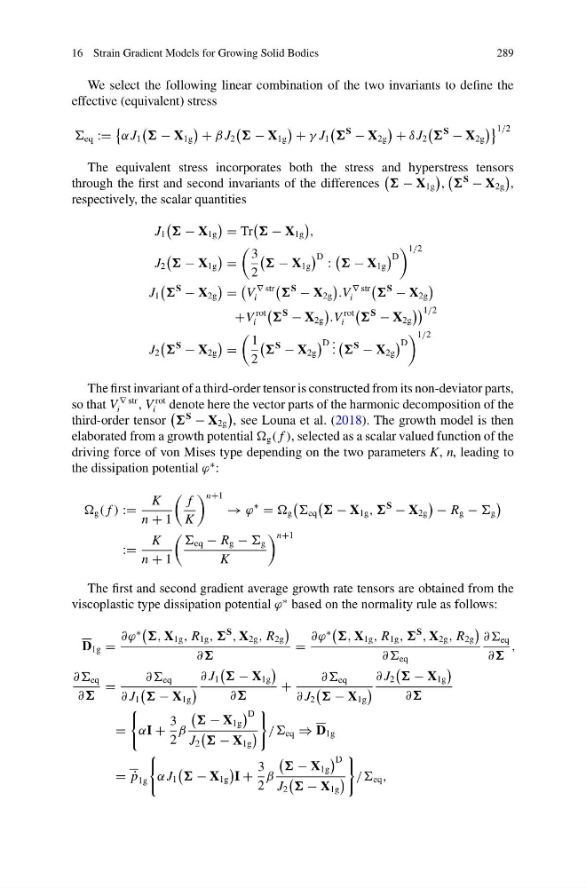
We select the following linear combination of the two invariants to define the
effective (equivalent) stress
eq :=
α J 1
− X 1g
+ β J 2
− X 1g
+ γ J 1
S
− X 2g
+ δ J 2
S
− X 2g
1/2
The equivalent stress incorporates both the stress and hyperstress tensors
through the first and second invariants of the differences
− X 1g
,
S
− X 2g
,
respectively, the scalar quantities
J 1
− X 1g
= Tr
− X 1g
,
J 2
− X 1g
=
3
2
− X 1g
D :
− X 1g
D
1/2
J 1
S
− X 2g
=
V
∇ str
i
S
− X 2g
.V
∇ str
i
S
− X 2g
+V
rot
i
S
− X 2g
.V
rot
i
S
− X 2g
1/2
J 2
S
− X 2g
=
1
2
S
− X 2g
D . . .
S
− X 2g
D
1/2
The first invariant of a third-order tensor is constructed from its non-deviator parts,
so that V
∇ str
i
, V
rot
i denote here the vector parts of the harmonic decomposition of the
third-order tensor
S
− X 2g
, see Louna et al. (2018). The growth model is then
elaborated from a growth potential g ( f ), selected as a scalar valued function of the
driving force of von Mises type depending on the two parameters K, n, leading to
the dissipation potential ϕ
∗ :
g ( f ) :=
K
n + 1
f
K
n+1
→ ϕ
∗
= g
eq
− X 1g ,
S
− X 2g
− R g − g
:=
K
n + 1
eq − R g − g
K
n+1
The first and second gradient average growth rate tensors are obtained from the
viscoplastic type dissipation potential ϕ
∗ based on the normality rule as follows:
D 1g =
∂ϕ
∗
, X 1g , R 1g ,
S
, X 2g , R 2g
∂
=
∂ϕ
∗
, X 1g , R 1g ,
S
, X 2g , R 2g
∂∂ eq
∂∂ eq
∂
,
∂∂ eq
∂
=
∂∂ eq
∂ J 1
− X 1g
∂ J 1
− X 1g
∂
+
∂∂ eq
∂ J 2
− X 1g
∂ J 2
− X 1g
∂
=
αI +
3
2
β
− X 1g
D
J 2
− X 1g
// eq ⇒ D 1g
= ˙
p 1g
α J 1
− X 1g
I +
3
2
β
− X 1g
D
J 2
− X 1g
// eq ,
289
We select the following linear combination of the two invariants to define the
effective (equivalent) stress
eq :=
α J 1
− X 1g
+ β J 2
− X 1g
+ γ J 1
S
− X 2g
+ δ J 2
S
− X 2g
1/2
The equivalent stress incorporates both the stress and hyperstress tensors
through the first and second invariants of the differences
− X 1g
,
S
− X 2g
,
respectively, the scalar quantities
J 1
− X 1g
= Tr
− X 1g
,
J 2
− X 1g
=
3
2
− X 1g
D :
− X 1g
D
1/2
J 1
S
− X 2g
=
V
∇ str
i
S
− X 2g
.V
∇ str
i
S
− X 2g
+V
rot
i
S
− X 2g
.V
rot
i
S
− X 2g
1/2
J 2
S
− X 2g
=
1
2
S
− X 2g
D . . .
S
− X 2g
D
1/2
The first invariant of a third-order tensor is constructed from its non-deviator parts,
so that V
∇ str
i
, V
rot
i denote here the vector parts of the harmonic decomposition of the
third-order tensor
S
− X 2g
, see Louna et al. (2018). The growth model is then
elaborated from a growth potential g ( f ), selected as a scalar valued function of the
driving force of von Mises type depending on the two parameters K, n, leading to
the dissipation potential ϕ
∗ :
g ( f ) :=
K
n + 1
f
K
n+1
→ ϕ
∗
= g
eq
− X 1g ,
S
− X 2g
− R g − g
:=
K
n + 1
eq − R g − g
K
n+1
The first and second gradient average growth rate tensors are obtained from the
viscoplastic type dissipation potential ϕ
∗ based on the normality rule as follows:
D 1g =
∂ϕ
∗
, X 1g , R 1g ,
S
, X 2g , R 2g
∂
=
∂ϕ
∗
, X 1g , R 1g ,
S
, X 2g , R 2g
∂∂ eq
∂∂ eq
∂
,
∂∂ eq
∂
=
∂∂ eq
∂ J 1
− X 1g
∂ J 1
− X 1g
∂
+
∂∂ eq
∂ J 2
− X 1g
∂ J 2
− X 1g
∂
=
αI +
3
2
β
− X 1g
D
J 2
− X 1g
// eq ⇒ D 1g
= ˙
p 1g
α J 1
− X 1g
I +
3
2
β
− X 1g
D
J 2
− X 1g
// eq ,