

16 Strain Gradient Models for Growing Solid Bodies
287
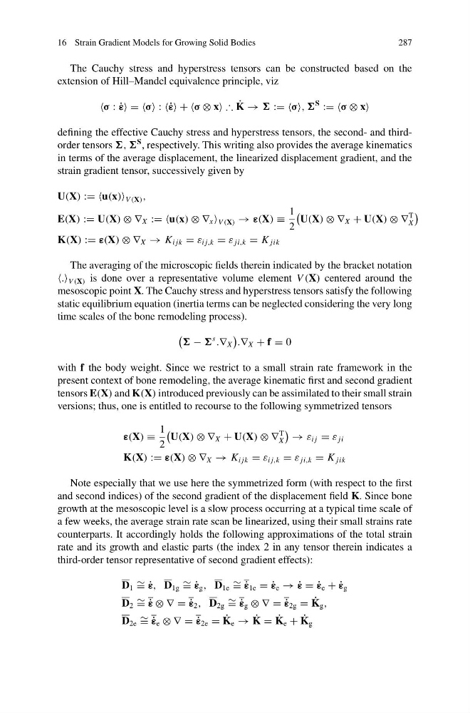
The Cauchy stress and hyperstress tensors can be constructed based on the
extension of Hill–Mandel equivalence principle, viz
σ : ˙
ε = σ : ˙ ε + σ ⊗ x ∴ ˙
K → := σ,
S
:= σ ⊗ x
defining the effective Cauchy stress and hyperstress tensors, the second- and thirdorder tensors ,
S , respectively. This writing also provides the average kinematics
in terms of the average displacement, the linearized displacement gradient, and the
strain gradient tensor, successively given by
U(X) := u(x) V (X) ,
E(X) := U(X) ⊗ ∇ X := u(x) ⊗ ∇ x V (X) → ε(X) ≡
1
2
U(X) ⊗ ∇ X + U(X) ⊗ ∇
T
X
K(X) := ε(X) ⊗ ∇ X → K i jk = ε i j,k = ε ji,k = K jik
The averaging of the microscopic fields therein indicated by the bracket notation
. V (X) is done over a representative volume element V (X) centered around the
mesoscopic point X. The Cauchy stress and hyperstress tensors satisfy the following
static equilibrium equation (inertia terms can be neglected considering the very long
time scales of the bone remodeling process).
−
s
.∇ X
.∇ X + f = 0
with f the body weight. Since we restrict to a small strain rate framework in the
present context of bone remodeling, the average kinematic first and second gradient
tensors E(X) and K(X) introduced previously can be assimilated to their small strain
versions; thus, one is entitled to recourse to the following symmetrized tensors
ε(X) ≡
1
2
U(X) ⊗ ∇ X + U(X) ⊗ ∇
T
X
→ ε i j = ε ji
K(X) := ε(X) ⊗ ∇ X → K i jk = ε i j,k = ε ji,k = K jik
Note especially that we use here the symmetrized form (with respect to the first
and second indices) of the second gradient of the displacement field K. Since bone
growth at the mesoscopic level is a slow process occurring at a typical time scale of
a few weeks, the average strain rate scan be linearized, using their small strains rate
counterparts. It accordingly holds the following approximations of the total strain
rate and its growth and elastic parts (the index 2 in any tensor therein indicates a
third-order tensor representative of second gradient effects):
D 1 ∼ = ˙
ε, D 1g ∼ = ˙
ε g , D 1e ∼ = ˙
ε 1e = ˙
ε e → ˙
ε = ˙
ε e + ˙
ε g
D 2 ∼ = ˙
ε ⊗ ∇ = ˙
ε 2 , D 2g ∼ = ˙
ε g ⊗ ∇ = ˙
ε 2g = ˙
K g ,
D 2e ∼ = ˙
ε e ⊗ ∇ = ˙
ε 2e = ˙
K e → ˙
K = ˙
K e + ˙
K g
287
The Cauchy stress and hyperstress tensors can be constructed based on the
extension of Hill–Mandel equivalence principle, viz
σ : ˙
ε = σ : ˙ ε + σ ⊗ x ∴ ˙
K → := σ,
S
:= σ ⊗ x
defining the effective Cauchy stress and hyperstress tensors, the second- and thirdorder tensors ,
S , respectively. This writing also provides the average kinematics
in terms of the average displacement, the linearized displacement gradient, and the
strain gradient tensor, successively given by
U(X) := u(x) V (X) ,
E(X) := U(X) ⊗ ∇ X := u(x) ⊗ ∇ x V (X) → ε(X) ≡
1
2
U(X) ⊗ ∇ X + U(X) ⊗ ∇
T
X
K(X) := ε(X) ⊗ ∇ X → K i jk = ε i j,k = ε ji,k = K jik
The averaging of the microscopic fields therein indicated by the bracket notation
. V (X) is done over a representative volume element V (X) centered around the
mesoscopic point X. The Cauchy stress and hyperstress tensors satisfy the following
static equilibrium equation (inertia terms can be neglected considering the very long
time scales of the bone remodeling process).
−
s
.∇ X
.∇ X + f = 0
with f the body weight. Since we restrict to a small strain rate framework in the
present context of bone remodeling, the average kinematic first and second gradient
tensors E(X) and K(X) introduced previously can be assimilated to their small strain
versions; thus, one is entitled to recourse to the following symmetrized tensors
ε(X) ≡
1
2
U(X) ⊗ ∇ X + U(X) ⊗ ∇
T
X
→ ε i j = ε ji
K(X) := ε(X) ⊗ ∇ X → K i jk = ε i j,k = ε ji,k = K jik
Note especially that we use here the symmetrized form (with respect to the first
and second indices) of the second gradient of the displacement field K. Since bone
growth at the mesoscopic level is a slow process occurring at a typical time scale of
a few weeks, the average strain rate scan be linearized, using their small strains rate
counterparts. It accordingly holds the following approximations of the total strain
rate and its growth and elastic parts (the index 2 in any tensor therein indicates a
third-order tensor representative of second gradient effects):
D 1 ∼ = ˙
ε, D 1g ∼ = ˙
ε g , D 1e ∼ = ˙
ε 1e = ˙
ε e → ˙
ε = ˙
ε e + ˙
ε g
D 2 ∼ = ˙
ε ⊗ ∇ = ˙
ε 2 , D 2g ∼ = ˙
ε g ⊗ ∇ = ˙
ε 2g = ˙
K g ,
D 2e ∼ = ˙
ε e ⊗ ∇ = ˙
ε 2e = ˙
K e → ˙
K = ˙
K e + ˙
K g