

13 High Strain Rate Tension Experiments Features …
215
F exp (t) = E T · S T · ε
T
(t)
(13.19)
where c I , c T are bar sound speeds of the incident (subscript I) and the transmission
(subscript T ) bars, E T and S T are Young modulus and cross-section area of output bar,
ε
I , ε
R and ε
T are incident, reflected, and transmitted pulses registered in measuring
bars.
The following iterative procedure for determination of the true diagram is to be
used:
1. The initial approximation of the material deformation diagram is selected (e.g.,
it can be a diagram obtained by extrapolation of a logarithmic curve, or an
ideal-plastic model) as a table.
2. Process of dynamic tension of a specimen is simulated according to the scheme
provided in Fig. 13.13, where boundary conditions at the top are V y (t) = V (t),
V x (t) = 0. Axial speed of the upper boundary V (t) is calculated by formula
(13.18).
3. The integrated reaction force F calc (t) on the fixed side is to be obtained.
4. Values (ε p
i , σ m
i ) are determined for a discrete set of times t i in a finite element
in which the maximum effective plastic strain is realized (a finite element on a
specimen’s axis in a minimum section). Here, ε p
i is an effective plastic strain in
the specified finite element, σ m
i is Mises stress in the specified finite element.
5. Tabular curve (
ε
i
p , σ
i
m ·
F exp (ti )
F calc( t i )
) is accepted as an approximation of a true strain
curve.
6. Steps 2–5 are repeated until the acceptable compliance of experimental and
simulated forces is obtained or diagram at the next step stops changing
significantly.
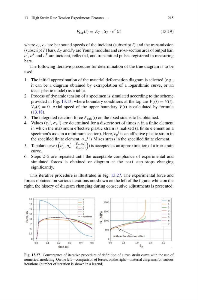
This iterative procedure is illustrated in Fig. 13.27. The experimental force and
forces obtained on various iterations are shown on the left of the figure, while on the
right, the history of diagram changing during consecutive adjustments is presented.
Fig. 13.27 Convergence of iterative procedure of definition of a true strain curve with the use of
numerical modeling. On the left—comparison of forces, on the right—material diagrams for various
iterations (number of iteration is shown in a legend)
215
F exp (t) = E T · S T · ε
T
(t)
(13.19)
where c I , c T are bar sound speeds of the incident (subscript I) and the transmission
(subscript T ) bars, E T and S T are Young modulus and cross-section area of output bar,
ε
I , ε
R and ε
T are incident, reflected, and transmitted pulses registered in measuring
bars.
The following iterative procedure for determination of the true diagram is to be
used:
1. The initial approximation of the material deformation diagram is selected (e.g.,
it can be a diagram obtained by extrapolation of a logarithmic curve, or an
ideal-plastic model) as a table.
2. Process of dynamic tension of a specimen is simulated according to the scheme
provided in Fig. 13.13, where boundary conditions at the top are V y (t) = V (t),
V x (t) = 0. Axial speed of the upper boundary V (t) is calculated by formula
(13.18).
3. The integrated reaction force F calc (t) on the fixed side is to be obtained.
4. Values (ε p
i , σ m
i ) are determined for a discrete set of times t i in a finite element
in which the maximum effective plastic strain is realized (a finite element on a
specimen’s axis in a minimum section). Here, ε p
i is an effective plastic strain in
the specified finite element, σ m
i is Mises stress in the specified finite element.
5. Tabular curve (
ε
i
p , σ
i
m ·
F exp (ti )
F calc( t i )
) is accepted as an approximation of a true strain
curve.
6. Steps 2–5 are repeated until the acceptable compliance of experimental and
simulated forces is obtained or diagram at the next step stops changing
significantly.
This iterative procedure is illustrated in Fig. 13.27. The experimental force and
forces obtained on various iterations are shown on the left of the figure, while on the
right, the history of diagram changing during consecutive adjustments is presented.
Fig. 13.27 Convergence of iterative procedure of definition of a true strain curve with the use of
numerical modeling. On the left—comparison of forces, on the right—material diagrams for various
iterations (number of iteration is shown in a legend)