

178
L. Igumnov et al.
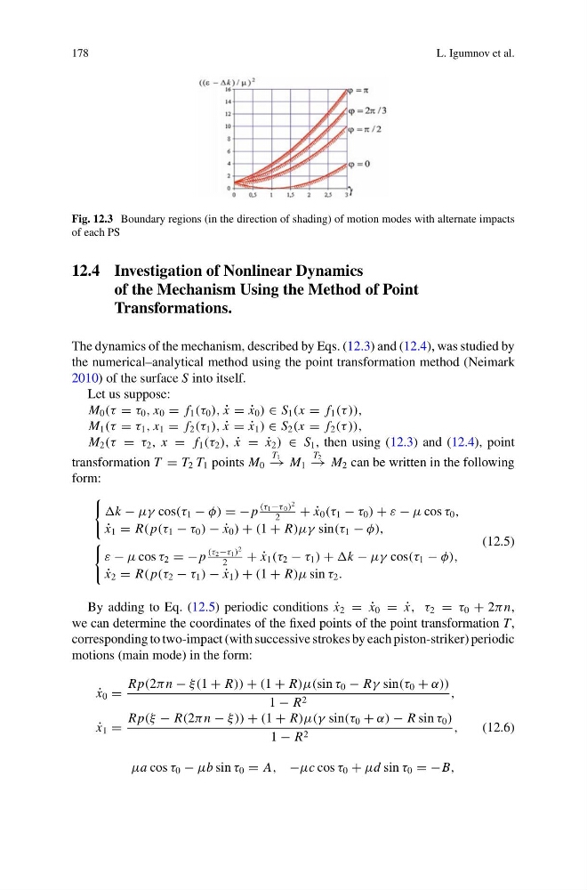
Fig. 12.3 Boundary regions (in the direction of shading) of motion modes with alternate impacts
of each PS
12.4 Investigation of Nonlinear Dynamics
of the Mechanism Using the Method of Point
Transformations.
The dynamics of the mechanism, described by Eqs. (12.3) and (12.4), was studied by
the numerical–analytical method using the point transformation method (Neimark
2010) of the surface S into itself.
Let us suppose:
M 0 (τ = τ 0 , x 0 = f 1 (τ 0 ), ˙
x = ˙
x 0 ) ∈ S 1 (x = f 1 (τ )),
M 1 (τ = τ 1 , x 1 = f 2 (τ 1 ), ˙
x = ˙
x 1 ) ∈ S 2 (x = f 2 (τ )),
M 2 (τ = τ 2 , x = f 1 (τ 2 ), ˙
x = ˙
x 2 ) ∈ S 1 , then using (12.3) and (12.4), point
transformation T = T 2 T 1 points M 0
T 1
− → M 1
T 2
− → M 2 can be written in the following
form:
k − μγ cos(τ 1 − φ) = −p
(τ 1 −τ 0 )
2
2
+ ˙
x 0 (τ 1 − τ 0 ) + ε − μ cos τ 0 ,
˙
x 1 = R( p(τ 1 − τ 0 ) − ˙
x 0 ) + (1 + R)μγ sin(τ 1 − φ),
ε − μ cos τ 2 = −p
(τ 2 −τ 1 )
2
2
+ ˙
x 1 (τ 2 − τ 1 ) + k − μγ cos(τ 1 − φ),
˙
x 2 = R( p(τ 2 − τ 1 ) − ˙
x 1 ) + (1 + R)μ sin τ 2 .
(12.5)
By adding to Eq. (12.5) periodic conditions ˙
x 2 = ˙
x 0 = ˙
x, τ 2 = τ 0 + 2π n,
we can determine the coordinates of the fixed points of the point transformation T,
corresponding to two-impact (with successive strokes by each piston-striker) periodic
motions (main mode) in the form:
˙
x 0 =
Rp(2π n − ξ(1 + R)) + (1 + R)μ(sin τ 0 − Rγ sin(τ 0 + α))
1 − R 2
,
˙
x 1 =
Rp(ξ − R(2π n − ξ)) + (1 + R)μ(γ sin(τ 0 + α) − R sin τ 0 )
1 − R 2
,
(12.6)
μa cos τ 0 − μb sin τ 0 = A, −μc cos τ 0 + μd sin τ 0 = −B,
L. Igumnov et al.
Fig. 12.3 Boundary regions (in the direction of shading) of motion modes with alternate impacts
of each PS
12.4 Investigation of Nonlinear Dynamics
of the Mechanism Using the Method of Point
Transformations.
The dynamics of the mechanism, described by Eqs. (12.3) and (12.4), was studied by
the numerical–analytical method using the point transformation method (Neimark
2010) of the surface S into itself.
Let us suppose:
M 0 (τ = τ 0 , x 0 = f 1 (τ 0 ), ˙
x = ˙
x 0 ) ∈ S 1 (x = f 1 (τ )),
M 1 (τ = τ 1 , x 1 = f 2 (τ 1 ), ˙
x = ˙
x 1 ) ∈ S 2 (x = f 2 (τ )),
M 2 (τ = τ 2 , x = f 1 (τ 2 ), ˙
x = ˙
x 2 ) ∈ S 1 , then using (12.3) and (12.4), point
transformation T = T 2 T 1 points M 0
T 1
− → M 1
T 2
− → M 2 can be written in the following
form:
k − μγ cos(τ 1 − φ) = −p
(τ 1 −τ 0 )
2
2
+ ˙
x 0 (τ 1 − τ 0 ) + ε − μ cos τ 0 ,
˙
x 1 = R( p(τ 1 − τ 0 ) − ˙
x 0 ) + (1 + R)μγ sin(τ 1 − φ),
ε − μ cos τ 2 = −p
(τ 2 −τ 1 )
2
2
+ ˙
x 1 (τ 2 − τ 1 ) + k − μγ cos(τ 1 − φ),
˙
x 2 = R( p(τ 2 − τ 1 ) − ˙
x 1 ) + (1 + R)μ sin τ 2 .
(12.5)
By adding to Eq. (12.5) periodic conditions ˙
x 2 = ˙
x 0 = ˙
x, τ 2 = τ 0 + 2π n,
we can determine the coordinates of the fixed points of the point transformation T,
corresponding to two-impact (with successive strokes by each piston-striker) periodic
motions (main mode) in the form:
˙
x 0 =
Rp(2π n − ξ(1 + R)) + (1 + R)μ(sin τ 0 − Rγ sin(τ 0 + α))
1 − R 2
,
˙
x 1 =
Rp(ξ − R(2π n − ξ)) + (1 + R)μ(γ sin(τ 0 + α) − R sin τ 0 )
1 − R 2
,
(12.6)
μa cos τ 0 − μb sin τ 0 = A, −μc cos τ 0 + μd sin τ 0 = −B,