

6 Construction of the Solutions of Non-stationary …
91
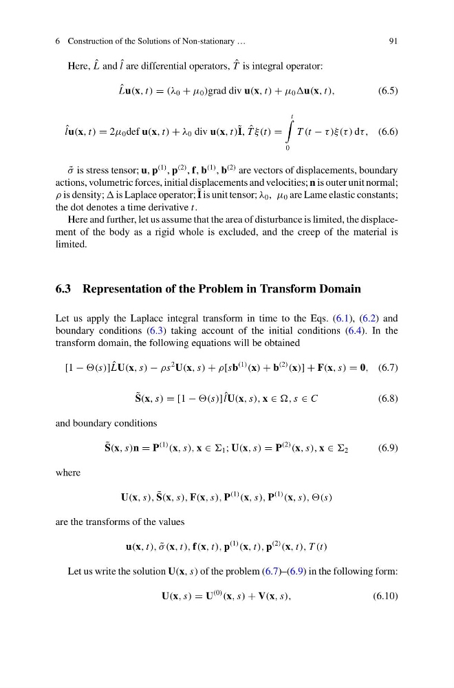
Here, ˆ
L and ˆ
l are differential operators, ˆ
T is integral operator:
ˆ
Lu(x, t) = (λ 0 + μ 0 )grad div u(x, t) + μ 0 u(x, t),
(6.5)
ˆ
lu(x, t) = 2μ 0 def u(x, t) + λ 0 div u(x, t) ˜
I, ˆ
T ξ(t) =
t
0
T (t − τ )ξ(τ ) dτ , (6.6)
˜
σ is stress tensor; u, p
(1) , p
(2) , f, b
(1) , b
(2) are vectors of displacements, boundary
actions, volumetric forces, initial displacements and velocities; n is outer unit normal;
ρ is density; is Laplace operator; ˜
I is unit tensor; λ 0 , μ 0 are Lame elastic constants;
the dot denotes a time derivative t.
Here and further, let us assume that the area of disturbance is limited, the displacement of the body as a rigid whole is excluded, and the creep of the material is
limited.
6.3 Representation of the Problem in Transform Domain
Let us apply the Laplace integral transform in time to the Eqs. (6.1), (6.2) and
boundary conditions (6.3) taking account of the initial conditions (6.4). In the
transform domain, the following equations will be obtained
[1 − (s)] ˆ
LU(x, s) − ρs
2 U(x, s) + ρ[sb
(1)
(x) + b
(2)
(x)] + F(x, s) = 0, (6.7)
˜
S(x, s) = [1 − (s)] ˆ
lU(x, s), x ∈ , s ∈ C
(6.8)
and boundary conditions
˜
S(x, s)n = P
(1)
(x, s), x ∈ 1 ; U(x, s) = P
(2)
(x, s), x ∈ 2
(6.9)
where
U(x, s), ˜
S(x, s), F(x, s), P
(1)
(x, s), P
(1)
(x, s), ,(s)
are the transforms of the values
u(x, t), ˜
σ (x, t), f(x, t), p
(1)
(x, t), p
(2)
(x, t), T (t)
Let us write the solution U(x, s) of the problem (6.7)–(6.9) in the following form:
U(x, s) = U
(0)
(x, s) + V(x, s),
(6.10)
91
Here, ˆ
L and ˆ
l are differential operators, ˆ
T is integral operator:
ˆ
Lu(x, t) = (λ 0 + μ 0 )grad div u(x, t) + μ 0 u(x, t),
(6.5)
ˆ
lu(x, t) = 2μ 0 def u(x, t) + λ 0 div u(x, t) ˜
I, ˆ
T ξ(t) =
t
0
T (t − τ )ξ(τ ) dτ , (6.6)
˜
σ is stress tensor; u, p
(1) , p
(2) , f, b
(1) , b
(2) are vectors of displacements, boundary
actions, volumetric forces, initial displacements and velocities; n is outer unit normal;
ρ is density; is Laplace operator; ˜
I is unit tensor; λ 0 , μ 0 are Lame elastic constants;
the dot denotes a time derivative t.
Here and further, let us assume that the area of disturbance is limited, the displacement of the body as a rigid whole is excluded, and the creep of the material is
limited.
6.3 Representation of the Problem in Transform Domain
Let us apply the Laplace integral transform in time to the Eqs. (6.1), (6.2) and
boundary conditions (6.3) taking account of the initial conditions (6.4). In the
transform domain, the following equations will be obtained
[1 − (s)] ˆ
LU(x, s) − ρs
2 U(x, s) + ρ[sb
(1)
(x) + b
(2)
(x)] + F(x, s) = 0, (6.7)
˜
S(x, s) = [1 − (s)] ˆ
lU(x, s), x ∈ , s ∈ C
(6.8)
and boundary conditions
˜
S(x, s)n = P
(1)
(x, s), x ∈ 1 ; U(x, s) = P
(2)
(x, s), x ∈ 2
(6.9)
where
U(x, s), ˜
S(x, s), F(x, s), P
(1)
(x, s), P
(1)
(x, s), ,(s)
are the transforms of the values
u(x, t), ˜
σ (x, t), f(x, t), p
(1)
(x, t), p
(2)
(x, t), T (t)
Let us write the solution U(x, s) of the problem (6.7)–(6.9) in the following form:
U(x, s) = U
(0)
(x, s) + V(x, s),
(6.10)