

92
L. Igumnov et al.
where U
(0)
(x, s) is the solution of a problem involving equations
ˆ
LU
(0)
(x, s) +
1
[1 − (s)]
{ρ[sb
(1)
(x) + b
(2)
(x)] + F(x, s)} = 0,
(6.11)
˜
S
(0)
(x, s) = ˆ
l U
(0)
(x, s), x ∈ , s ∈ C
(6.12)
and boundary conditions
˜
S
(0)
(x, s)n =
P
(1)
(x, s)
1 − (s)
, x ∈ 1 ; U
(0)
(x, s) = P
(2)
(x, s), x ∈ 2
(6.13)
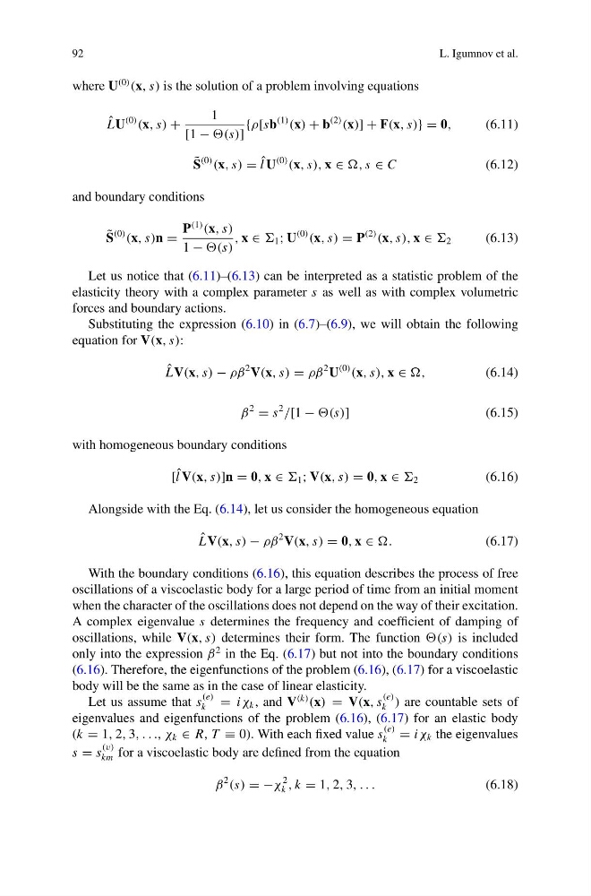
Let us notice that (6.11)–(6.13) can be interpreted as a statistic problem of the
elasticity theory with a complex parameter s as well as with complex volumetric
forces and boundary actions.
Substituting the expression (6.10) in (6.7)–(6.9), we will obtain the following
equation for V(x, s):
ˆ
LV(x, s) − ρβ
2 V(x, s) = ρβ
2 U
(0)
(x, s), x ∈ ,
(6.14)
β
2
= s
2
/[1 − (s)]
(6.15)
with homogeneous boundary conditions
[ ˆ
l V(x, s)]n = 0, x ∈ 1 ; V(x, s) = 0, x ∈ 2
(6.16)
Alongside with the Eq. (6.14), let us consider the homogeneous equation
ˆ
LV(x, s) − ρβ
2 V(x, s) = 0, x ∈ .
(6.17)
With the boundary conditions (6.16), this equation describes the process of free
oscillations of a viscoelastic body for a large period of time from an initial moment
when the character of the oscillations does not depend on the way of their excitation.
A complex eigenvalue s determines the frequency and coefficient of damping of
oscillations, while V(x, s) determines their form. The function (s) is included
only into the expression β
2 in the Eq. (6.17) but not into the boundary conditions
(6.16). Therefore, the eigenfunctions of the problem (6.16), (6.17) for a viscoelastic
body will be the same as in the case of linear elasticity.
Let us assume that s
(e)
k
= iχ k , and V
(k)
(x) = V(x, s
(e)
k ) are countable sets of
eigenvalues and eigenfunctions of the problem (6.16), (6.17) for an elastic body
(k = 1, 2, 3, . . ., χ k ∈ R, T ≡ 0). With each fixed value s
(e)
k = iχ k the eigenvalues
s = s
(v)
km for a viscoelastic body are defined from the equation
β
2
(s) = −χ
2
k , k = 1, 2, 3, . . .
(6.18)
L. Igumnov et al.
where U
(0)
(x, s) is the solution of a problem involving equations
ˆ
LU
(0)
(x, s) +
1
[1 − (s)]
{ρ[sb
(1)
(x) + b
(2)
(x)] + F(x, s)} = 0,
(6.11)
˜
S
(0)
(x, s) = ˆ
l U
(0)
(x, s), x ∈ , s ∈ C
(6.12)
and boundary conditions
˜
S
(0)
(x, s)n =
P
(1)
(x, s)
1 − (s)
, x ∈ 1 ; U
(0)
(x, s) = P
(2)
(x, s), x ∈ 2
(6.13)
Let us notice that (6.11)–(6.13) can be interpreted as a statistic problem of the
elasticity theory with a complex parameter s as well as with complex volumetric
forces and boundary actions.
Substituting the expression (6.10) in (6.7)–(6.9), we will obtain the following
equation for V(x, s):
ˆ
LV(x, s) − ρβ
2 V(x, s) = ρβ
2 U
(0)
(x, s), x ∈ ,
(6.14)
β
2
= s
2
/[1 − (s)]
(6.15)
with homogeneous boundary conditions
[ ˆ
l V(x, s)]n = 0, x ∈ 1 ; V(x, s) = 0, x ∈ 2
(6.16)
Alongside with the Eq. (6.14), let us consider the homogeneous equation
ˆ
LV(x, s) − ρβ
2 V(x, s) = 0, x ∈ .
(6.17)
With the boundary conditions (6.16), this equation describes the process of free
oscillations of a viscoelastic body for a large period of time from an initial moment
when the character of the oscillations does not depend on the way of their excitation.
A complex eigenvalue s determines the frequency and coefficient of damping of
oscillations, while V(x, s) determines their form. The function (s) is included
only into the expression β
2 in the Eq. (6.17) but not into the boundary conditions
(6.16). Therefore, the eigenfunctions of the problem (6.16), (6.17) for a viscoelastic
body will be the same as in the case of linear elasticity.
Let us assume that s
(e)
k
= iχ k , and V
(k)
(x) = V(x, s
(e)
k ) are countable sets of
eigenvalues and eigenfunctions of the problem (6.16), (6.17) for an elastic body
(k = 1, 2, 3, . . ., χ k ∈ R, T ≡ 0). With each fixed value s
(e)
k = iχ k the eigenvalues
s = s
(v)
km for a viscoelastic body are defined from the equation
β
2
(s) = −χ
2
k , k = 1, 2, 3, . . .
(6.18)