

167
sense to measure penalty Z in the same units as that of cost ($). We
then define a locally linear penalty function
3 Z:
Z C
m
= + α
(5.8)
or
m
C
Z
= −
+
1
1
α
α
(5.9)
Here α is the change in Z associated with unit increase in m and
has the units of $/kg. Equation 5.9 defines a linear a relationship
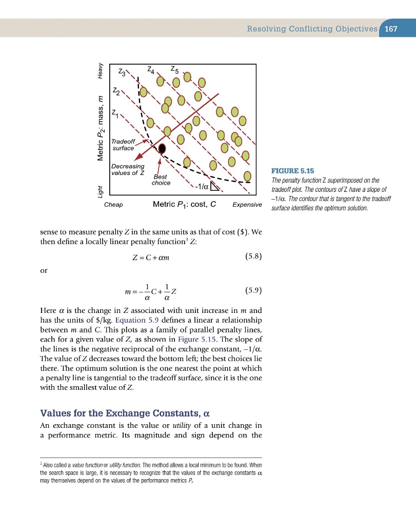
between m and C. This plots as a family of parallel penalty lines,
each for a given value of Z, as shown in Figure 5.15. The slope of
the lines is the negative reciprocal of the exchange constant, −1/α.
The value of Z decreases toward the bottom left; the best choices lie
there. The optimum solution is the one nearest the point at which
a penalty line is tangential to the tradeoff surface, since it is the one
with the smallest value of Z.
values for the exchange Constants, α
An exchange constant is the value or utility of a unit change in
a performance metric. Its magnitude and sign depend on the
Figure 5.15
The penalty function Z superimposed on the
tradeoff plot. The contours of Z have a slope of
−1/α. The contour that is tangent to the tradeoff
surface identifies the optimum solution.
Best
choice
Decreasing
values of Z
Tradeoff
surface
Z
1
Z 2
Z 3
Z 5
Z 4
-1/α
Cheap
Metric P 1 : cost, C
Expensive
Light
Metric P
2 : mass, m
Heavy
3 Also called a value function or utility function. The method allows a local minimum to be found. When
the search space is large, it is necessary to recognize that the values of the exchange constants α i
may themselves depend on the values of the performance metrics P i .
Resolving Conflicting Objectives
sense to measure penalty Z in the same units as that of cost ($). We
then define a locally linear penalty function
3 Z:
Z C
m
= + α
(5.8)
or
m
C
Z
= −
+
1
1
α
α
(5.9)
Here α is the change in Z associated with unit increase in m and
has the units of $/kg. Equation 5.9 defines a linear a relationship
between m and C. This plots as a family of parallel penalty lines,
each for a given value of Z, as shown in Figure 5.15. The slope of
the lines is the negative reciprocal of the exchange constant, −1/α.
The value of Z decreases toward the bottom left; the best choices lie
there. The optimum solution is the one nearest the point at which
a penalty line is tangential to the tradeoff surface, since it is the one
with the smallest value of Z.
values for the exchange Constants, α
An exchange constant is the value or utility of a unit change in
a performance metric. Its magnitude and sign depend on the
Figure 5.15
The penalty function Z superimposed on the
tradeoff plot. The contours of Z have a slope of
−1/α. The contour that is tangent to the tradeoff
surface identifies the optimum solution.
Best
choice
Decreasing
values of Z
Tradeoff
surface
Z
1
Z 2
Z 3
Z 5
Z 4
-1/α
Cheap
Metric P 1 : cost, C
Expensive
Light
Metric P
2 : mass, m
Heavy
3 Also called a value function or utility function. The method allows a local minimum to be found. When
the search space is large, it is necessary to recognize that the values of the exchange constants α i
may themselves depend on the values of the performance metrics P i .
Resolving Conflicting Objectives