

C haPter 5 Material Property Charts and their Uses
166
tions like those at B have the characteristic that no other solutions
exist with lower values of both P 1 and P 2 . These are said to be
nondominated solutions. The line or surface on which they lie is
called the nondominated or optimal tradeoff surface. The values of
P 1 and P 2 corresponding to the nondominated set of solutions are
called the Pareto set.
There are three strategies for progressing further. The solutions on or
near the tradeoff surface offer the best compromise; the rest can be
rejected. Often this is enough to identify a shortlist, using intuition
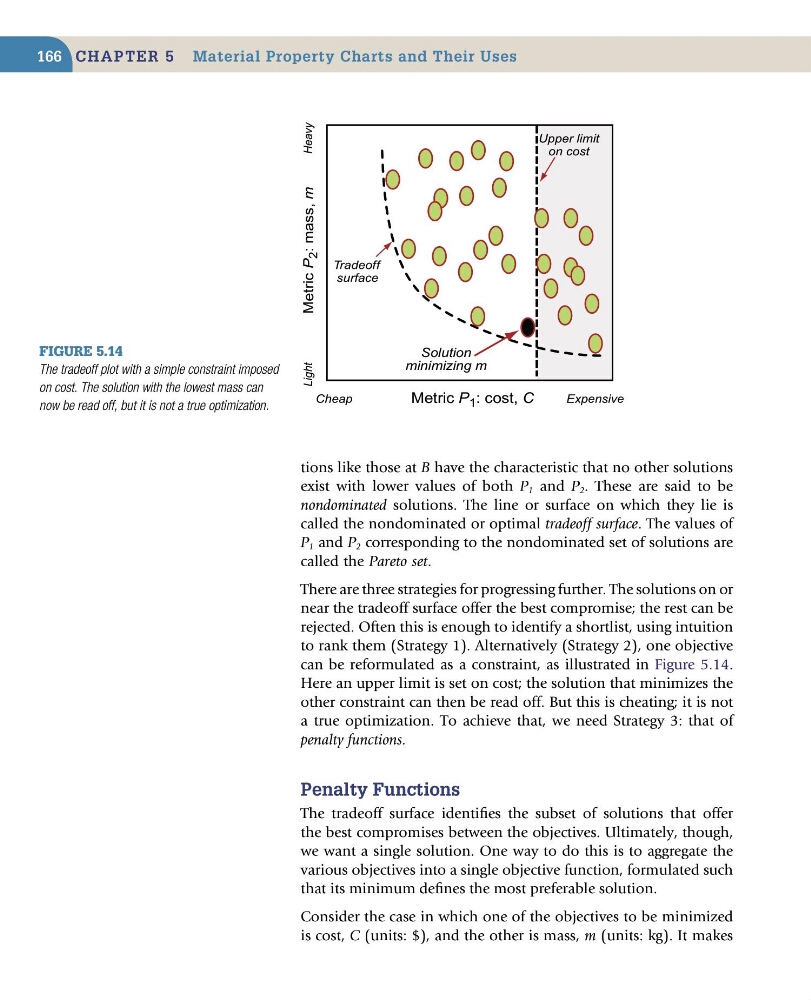
to rank them (Strategy 1). Alternatively (Strategy 2), one objective
can be reformulated as a constraint, as illustrated in Figure 5.14.
Here an upper limit is set on cost; the solution that minimizes the
other constraint can then be read off. But this is cheating; it is not
a true optimization. To achieve that, we need Strategy 3: that of
penalty functions.
Penalty Functions
The tradeoff surface identifies the subset of solutions that offer
the best compromises between the objectives. Ultimately, though,
we want a single solution. One way to do this is to aggregate the
various objectives into a single objective function, formulated such
that its minimum defines the most preferable solution.
Consider the case in which one of the objectives to be minimized
is cost, C (units: $), and the other is mass, m (units: kg). It makes
Figure 5.14
The tradeoff plot with a simple constraint imposed
on cost. The solution with the lowest mass can
now be read off, but it is not a true optimization.
Solution
minimizing m
Tradeoff
surface
Upper limit
on cost
Cheap
Metric P 1 : cost, C
Expensive
Light
Metric P
2 : mass, m
Heavy
166
tions like those at B have the characteristic that no other solutions
exist with lower values of both P 1 and P 2 . These are said to be
nondominated solutions. The line or surface on which they lie is
called the nondominated or optimal tradeoff surface. The values of
P 1 and P 2 corresponding to the nondominated set of solutions are
called the Pareto set.
There are three strategies for progressing further. The solutions on or
near the tradeoff surface offer the best compromise; the rest can be
rejected. Often this is enough to identify a shortlist, using intuition
to rank them (Strategy 1). Alternatively (Strategy 2), one objective
can be reformulated as a constraint, as illustrated in Figure 5.14.
Here an upper limit is set on cost; the solution that minimizes the
other constraint can then be read off. But this is cheating; it is not
a true optimization. To achieve that, we need Strategy 3: that of
penalty functions.
Penalty Functions
The tradeoff surface identifies the subset of solutions that offer
the best compromises between the objectives. Ultimately, though,
we want a single solution. One way to do this is to aggregate the
various objectives into a single objective function, formulated such
that its minimum defines the most preferable solution.
Consider the case in which one of the objectives to be minimized
is cost, C (units: $), and the other is mass, m (units: kg). It makes
Figure 5.14
The tradeoff plot with a simple constraint imposed
on cost. The solution with the lowest mass can
now be read off, but it is not a true optimization.
Solution
minimizing m
Tradeoff
surface
Upper limit
on cost
Cheap
Metric P 1 : cost, C
Expensive
Light
Metric P
2 : mass, m
Heavy