

3 Uncertainty Quantification in Lasso-Type Regularization Problems
91
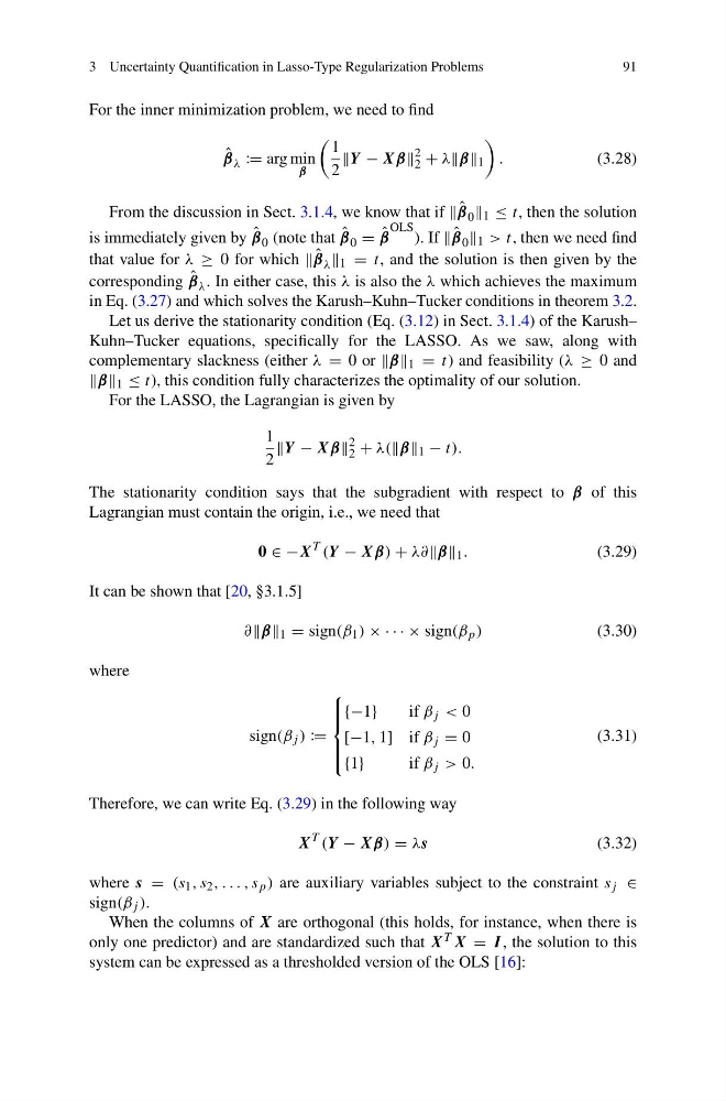
For the inner minimization problem, we need to find
ˆ
β λ := arg min
β
1
2
Y − Xβ
2
2 + λβ 1
.
(3.28)
From the discussion in Sect. 3.1.4, we know that if ˆ
β 0 1 ≤ t, then the solution
is immediately given by ˆ
β 0 (note that ˆ
β 0 = ˆ
β
OLS ). If ˆ
β 0 1 > t, then we need find
that value for λ ≥ 0 for which ˆ
β λ 1 = t, and the solution is then given by the
corresponding ˆ
β λ . In either case, this λ is also the λ which achieves the maximum
in Eq. (3.27) and which solves the Karush–Kuhn–Tucker conditions in theorem 3.2.
Let us derive the stationarity condition (Eq. (3.12) in Sect. 3.1.4) of the Karush–
Kuhn–Tucker equations, specifically for the LASSO. As we saw, along with
complementary slackness (either λ = 0 or β 1 = t) and feasibility (λ ≥ 0 and
β 1 ≤ t), this condition fully characterizes the optimality of our solution.
For the LASSO, the Lagrangian is given by
1
2
Y − Xβ
2
2 + λ(β 1 − t).
The stationarity condition says that the subgradient with respect to β of this
Lagrangian must contain the origin, i.e., we need that
0 ∈ −X
T (Y − Xβ) + λ∂β 1 .
(3.29)
It can be shown that [20, §3.1.5]
∂β 1 = sign(β 1 ) × · · · × sign(β p )
(3.30)
where
sign(β j ) :=
⎧
⎪ ⎪ ⎨
⎪ ⎪ ⎩
{−1}
if β j < 0
[−1, 1] if β j = 0
{1}
if β j > 0.
(3.31)
Therefore, we can write Eq. (3.29) in the following way
X
T (Y − Xβ) = λs
(3.32)
where s = (s 1 , s 2 , . . . , s p ) are auxiliary variables subject to the constraint s j ∈
sign(β j ).
When the columns of X are orthogonal (this holds, for instance, when there is
only one predictor) and are standardized such that X T X = I , the solution to this
system can be expressed as a thresholded version of the OLS [16]:
91
For the inner minimization problem, we need to find
ˆ
β λ := arg min
β
1
2
Y − Xβ
2
2 + λβ 1
.
(3.28)
From the discussion in Sect. 3.1.4, we know that if ˆ
β 0 1 ≤ t, then the solution
is immediately given by ˆ
β 0 (note that ˆ
β 0 = ˆ
β
OLS ). If ˆ
β 0 1 > t, then we need find
that value for λ ≥ 0 for which ˆ
β λ 1 = t, and the solution is then given by the
corresponding ˆ
β λ . In either case, this λ is also the λ which achieves the maximum
in Eq. (3.27) and which solves the Karush–Kuhn–Tucker conditions in theorem 3.2.
Let us derive the stationarity condition (Eq. (3.12) in Sect. 3.1.4) of the Karush–
Kuhn–Tucker equations, specifically for the LASSO. As we saw, along with
complementary slackness (either λ = 0 or β 1 = t) and feasibility (λ ≥ 0 and
β 1 ≤ t), this condition fully characterizes the optimality of our solution.
For the LASSO, the Lagrangian is given by
1
2
Y − Xβ
2
2 + λ(β 1 − t).
The stationarity condition says that the subgradient with respect to β of this
Lagrangian must contain the origin, i.e., we need that
0 ∈ −X
T (Y − Xβ) + λ∂β 1 .
(3.29)
It can be shown that [20, §3.1.5]
∂β 1 = sign(β 1 ) × · · · × sign(β p )
(3.30)
where
sign(β j ) :=
⎧
⎪ ⎪ ⎨
⎪ ⎪ ⎩
{−1}
if β j < 0
[−1, 1] if β j = 0
{1}
if β j > 0.
(3.31)
Therefore, we can write Eq. (3.29) in the following way
X
T (Y − Xβ) = λs
(3.32)
where s = (s 1 , s 2 , . . . , s p ) are auxiliary variables subject to the constraint s j ∈
sign(β j ).
When the columns of X are orthogonal (this holds, for instance, when there is
only one predictor) and are standardized such that X T X = I , the solution to this
system can be expressed as a thresholded version of the OLS [16]: