

90
T. Basu et al.
q=2
q=1
q=0.5
q=0.01
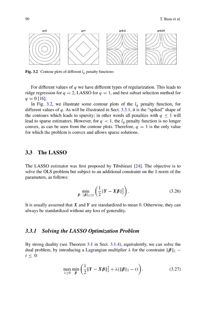
Fig. 3.2 Contour plots of different l q penalty functions
For different values of q we have different types of regularization. This leads to
ridge regression for q = 2, LASSO for q = 1, and best subset selection method for
q = 0 [16].
In Fig. 3.2, we illustrate some contour plots of the l q penalty function, for
different values of q. As will be illustrated in Sect. 3.3.1, it is the “spiked” shape of
the contours which leads to sparsity; in other words all penalties with q ≤ 1 will
lead to sparse estimators. However, for q < 1, the l q penalty function is no longer
convex, as can be seen from the contour plots. Therefore, q = 1 is the only value
for which the problem is convex and allows sparse solutions.
3.3 The LASSO
The LASSO estimator was first proposed by Tibshirani [24]. The objective is to
solve the OLS problem but subject to an additional constraint on the 1-norm of the
parameters, as follows:
min
β : :β 1 ≤t
1
2
Y − Xβ
2
2
.
(3.26)
It is usually assumed that X and Y are standardized to mean 0. Otherwise, they can
always be standardized without any loss of generality.
3.3.1 Solving the LASSO Optimization Problem
By strong duality (see Theorem 3.1 in Sect. 3.1.4), equivalently, we can solve the
dual problem, by introducing a Lagrangian multiplier λ for the constraint β 1 −
t ≤ 0:
max
λ≥0
min
β
1
2
Y − Xβ
2
2 + λ(β 1 − t)
.
(3.27)
T. Basu et al.
q=2
q=1
q=0.5
q=0.01
Fig. 3.2 Contour plots of different l q penalty functions
For different values of q we have different types of regularization. This leads to
ridge regression for q = 2, LASSO for q = 1, and best subset selection method for
q = 0 [16].
In Fig. 3.2, we illustrate some contour plots of the l q penalty function, for
different values of q. As will be illustrated in Sect. 3.3.1, it is the “spiked” shape of
the contours which leads to sparsity; in other words all penalties with q ≤ 1 will
lead to sparse estimators. However, for q < 1, the l q penalty function is no longer
convex, as can be seen from the contour plots. Therefore, q = 1 is the only value
for which the problem is convex and allows sparse solutions.
3.3 The LASSO
The LASSO estimator was first proposed by Tibshirani [24]. The objective is to
solve the OLS problem but subject to an additional constraint on the 1-norm of the
parameters, as follows:
min
β : :β 1 ≤t
1
2
Y − Xβ
2
2
.
(3.26)
It is usually assumed that X and Y are standardized to mean 0. Otherwise, they can
always be standardized without any loss of generality.
3.3.1 Solving the LASSO Optimization Problem
By strong duality (see Theorem 3.1 in Sect. 3.1.4), equivalently, we can solve the
dual problem, by introducing a Lagrangian multiplier λ for the constraint β 1 −
t ≤ 0:
max
λ≥0
min
β
1
2
Y − Xβ
2
2 + λ(β 1 − t)
.
(3.27)