

3 Uncertainty Quantification in Lasso-Type Regularization Problems
89
ˆ
c λ = arg min
c≥0
Y − XC ˆ
β
OLS
2
2 + λc 1
(3.22)
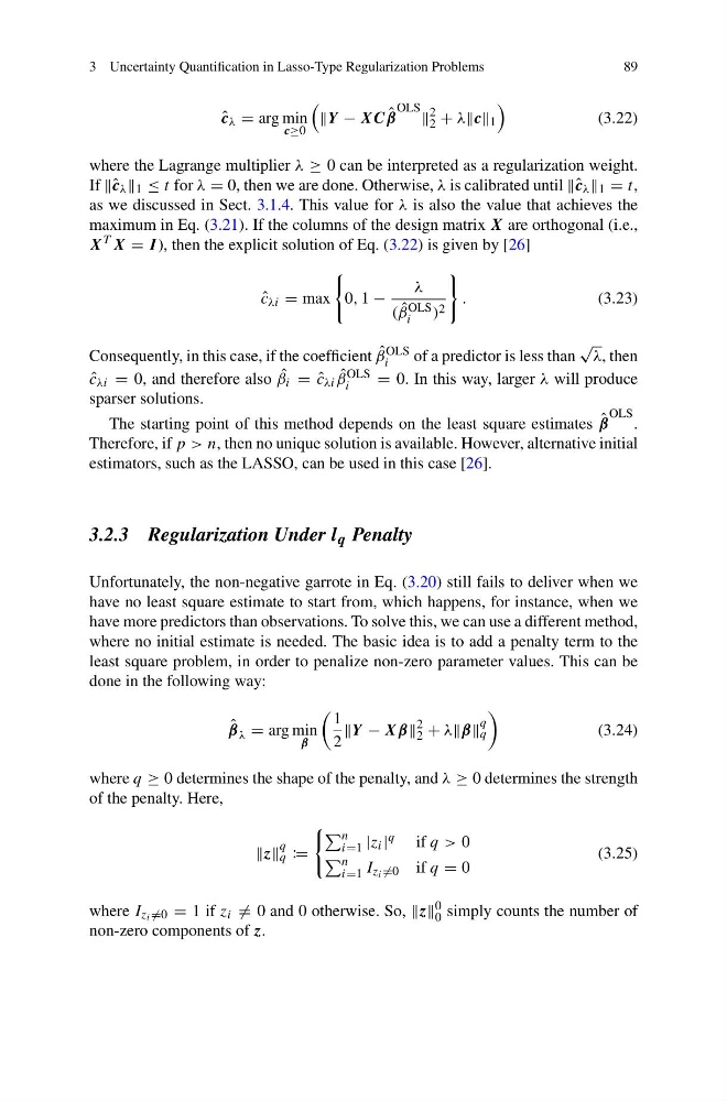
where the Lagrange multiplier λ ≥ 0 can be interpreted as a regularization weight.
If ˆ c λ 1 ≤ t for λ = 0, then we are done. Otherwise, λ is calibrated until ˆ c λ 1 = t,
as we discussed in Sect. 3.1.4. This value for λ is also the value that achieves the
maximum in Eq. (3.21). If the columns of the design matrix X are orthogonal (i.e.,
X T X = I ), then the explicit solution of Eq. (3.22) is given by [26]
ˆ
c λi = max
0, 1 −
λ
( ˆ
β OLS
i
) 2
.
(3.23)
Consequently, in this case, if the coefficient ˆ
β OLS
i
of a predictor is less than
√
λ, then
ˆ
c λi = 0, and therefore also ˆ
β i = ˆ
c λi ˆ
β OLS
i
= 0. In this way, larger λ will produce
sparser solutions.
The starting point of this method depends on the least square estimates ˆ
β
OLS .
Therefore, if p > n, then no unique solution is available. However, alternative initial
estimators, such as the LASSO, can be used in this case [26].
3.2.3 Regularization Under l q Penalty
Unfortunately, the non-negative garrote in Eq. (3.20) still fails to deliver when we
have no least square estimate to start from, which happens, for instance, when we
have more predictors than observations. To solve this, we can use a different method,
where no initial estimate is needed. The basic idea is to add a penalty term to the
least square problem, in order to penalize non-zero parameter values. This can be
done in the following way:
ˆ
β λ = arg min
β
1
2
Y − Xβ
2
2 + λβ
q
q
(3.24)
where q ≥ 0 determines the shape of the penalty, and λ ≥ 0 determines the strength
of the penalty. Here,
z
q
q :=
n
i=1 |z i | q if q > 0
n
i=1 I z i =0 if q = 0
(3.25)
where I z i =0 = 1 if z i = 0 and 0 otherwise. So, z 0
0 simply counts the number of
non-zero components of z.
89
ˆ
c λ = arg min
c≥0
Y − XC ˆ
β
OLS
2
2 + λc 1
(3.22)
where the Lagrange multiplier λ ≥ 0 can be interpreted as a regularization weight.
If ˆ c λ 1 ≤ t for λ = 0, then we are done. Otherwise, λ is calibrated until ˆ c λ 1 = t,
as we discussed in Sect. 3.1.4. This value for λ is also the value that achieves the
maximum in Eq. (3.21). If the columns of the design matrix X are orthogonal (i.e.,
X T X = I ), then the explicit solution of Eq. (3.22) is given by [26]
ˆ
c λi = max
0, 1 −
λ
( ˆ
β OLS
i
) 2
.
(3.23)
Consequently, in this case, if the coefficient ˆ
β OLS
i
of a predictor is less than
√
λ, then
ˆ
c λi = 0, and therefore also ˆ
β i = ˆ
c λi ˆ
β OLS
i
= 0. In this way, larger λ will produce
sparser solutions.
The starting point of this method depends on the least square estimates ˆ
β
OLS .
Therefore, if p > n, then no unique solution is available. However, alternative initial
estimators, such as the LASSO, can be used in this case [26].
3.2.3 Regularization Under l q Penalty
Unfortunately, the non-negative garrote in Eq. (3.20) still fails to deliver when we
have no least square estimate to start from, which happens, for instance, when we
have more predictors than observations. To solve this, we can use a different method,
where no initial estimate is needed. The basic idea is to add a penalty term to the
least square problem, in order to penalize non-zero parameter values. This can be
done in the following way:
ˆ
β λ = arg min
β
1
2
Y − Xβ
2
2 + λβ
q
q
(3.24)
where q ≥ 0 determines the shape of the penalty, and λ ≥ 0 determines the strength
of the penalty. Here,
z
q
q :=
n
i=1 |z i | q if q > 0
n
i=1 I z i =0 if q = 0
(3.25)
where I z i =0 = 1 if z i = 0 and 0 otherwise. So, z 0
0 simply counts the number of
non-zero components of z.