

92
T. Basu et al.
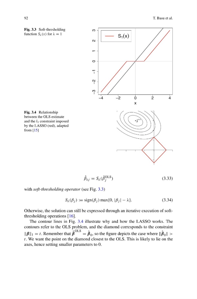
Fig. 3.3 Soft-thresholding
function S λ (x) for λ = 1
−4
−2
0
2
4
−3 −2 −1
0
1
2
3
x
S 1 (x)
Fig. 3.4 Relationship
between the OLS estimate
and the l 1 constraint imposed
by the LASSO (red), adapted
from [15]
l β
^ OLS
ˆ
β λj = S λ ( ˆ
β
OLS
j
)
(3.33)
with soft-thresholding operator (see Fig. 3.3)
S λ (β j ) := sign(β j ) max{0, |β j | − λ}.
(3.34)
Otherwise, the solution can still be expressed through an iterative execution of softthresholding operations [16].
The contour lines in Fig. 3.4 illustrate why and how the LASSO works. The
contours refer to the OLS problem, and the diamond corresponds to the constraint
β 1 = t. Remember that ˆ
β
OLS = ˆ
β 0 , so the figure depicts the case where ˆ
β 0 >
t. We want the point on the diamond closest to the OLS. This is likely to lie on the
axes, hence setting smaller parameters to 0.
T. Basu et al.
Fig. 3.3 Soft-thresholding
function S λ (x) for λ = 1
−4
−2
0
2
4
−3 −2 −1
0
1
2
3
x
S 1 (x)
Fig. 3.4 Relationship
between the OLS estimate
and the l 1 constraint imposed
by the LASSO (red), adapted
from [15]
l β
^ OLS
ˆ
β λj = S λ ( ˆ
β
OLS
j
)
(3.33)
with soft-thresholding operator (see Fig. 3.3)
S λ (β j ) := sign(β j ) max{0, |β j | − λ}.
(3.34)
Otherwise, the solution can still be expressed through an iterative execution of softthresholding operations [16].
The contour lines in Fig. 3.4 illustrate why and how the LASSO works. The
contours refer to the OLS problem, and the diamond corresponds to the constraint
β 1 = t. Remember that ˆ
β
OLS = ˆ
β 0 , so the figure depicts the case where ˆ
β 0 >
t. We want the point on the diamond closest to the OLS. This is likely to lie on the
axes, hence setting smaller parameters to 0.