

15 In-flight Icing: Modeling, Prediction, and Uncertainty
491
u(x) =
⎧
⎪ ⎪ ⎪ ⎪ ⎪ ⎨
⎪ ⎪ ⎪ ⎪ ⎪ ⎩
N
i=1
w i (x)U i
N
i=1
w i (x)
,
if d(x, x i ) = 0
u i ,
if d(x, x i ) = 0,
(15.41)
where w i (x) =
1
d(x, x i ) p is a weighting function as defined by Shepard [89] and
d(x, x i ) represents the distance between the points x and x i .
15.3.6 Numerical Results
The numerical results of the different fidelity levels of ice accretion simulations
will now be compared against experimental data. These will also be displayed
throughout the different ice regimes where different ice shapes are present and for
large ice accretion time. Gori et al. [60] have demonstrated this with results from
the PoliMIce solver resembling closely to experimental data.
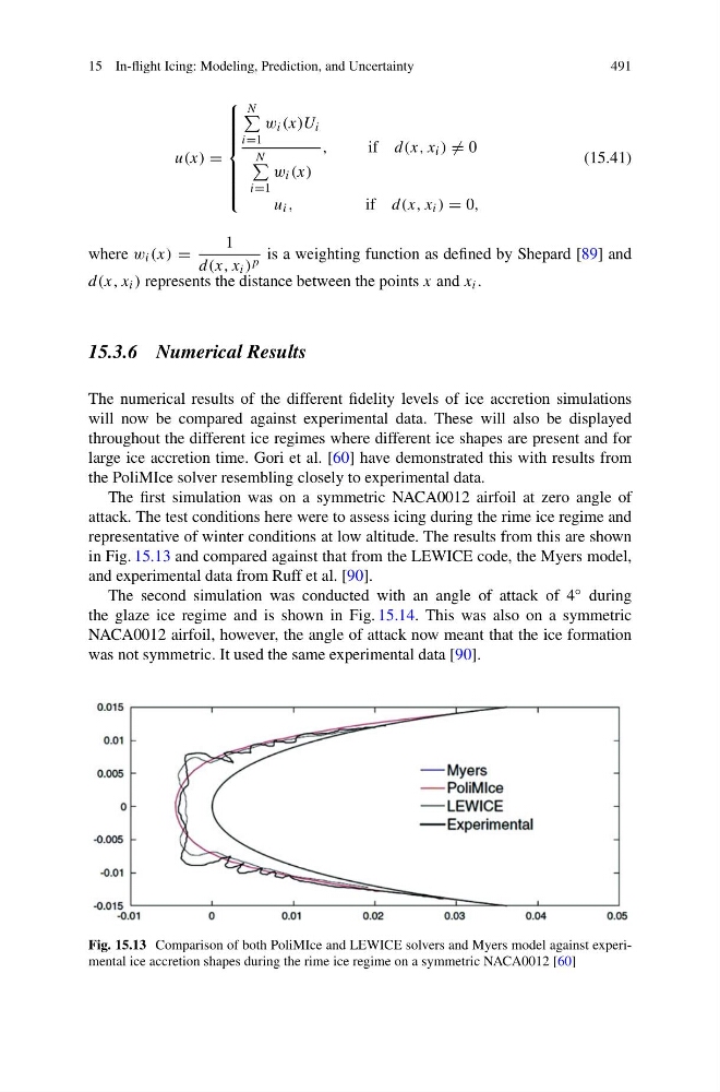
The first simulation was on a symmetric NACA0012 airfoil at zero angle of
attack. The test conditions here were to assess icing during the rime ice regime and
representative of winter conditions at low altitude. The results from this are shown
in Fig. 15.13 and compared against that from the LEWICE code, the Myers model,
and experimental data from Ruff et al. [90].
The second simulation was conducted with an angle of attack of 4 ◦ during
the glaze ice regime and is shown in Fig. 15.14. This was also on a symmetric
NACA0012 airfoil, however, the angle of attack now meant that the ice formation
was not symmetric. It used the same experimental data [90].
Fig. 15.13 Comparison of both PoliMIce and LEWICE solvers and Myers model against experimental ice accretion shapes during the rime ice regime on a symmetric NACA0012 [60]
491
u(x) =
⎧
⎪ ⎪ ⎪ ⎪ ⎪ ⎨
⎪ ⎪ ⎪ ⎪ ⎪ ⎩
N
i=1
w i (x)U i
N
i=1
w i (x)
,
if d(x, x i ) = 0
u i ,
if d(x, x i ) = 0,
(15.41)
where w i (x) =
1
d(x, x i ) p is a weighting function as defined by Shepard [89] and
d(x, x i ) represents the distance between the points x and x i .
15.3.6 Numerical Results
The numerical results of the different fidelity levels of ice accretion simulations
will now be compared against experimental data. These will also be displayed
throughout the different ice regimes where different ice shapes are present and for
large ice accretion time. Gori et al. [60] have demonstrated this with results from
the PoliMIce solver resembling closely to experimental data.
The first simulation was on a symmetric NACA0012 airfoil at zero angle of
attack. The test conditions here were to assess icing during the rime ice regime and
representative of winter conditions at low altitude. The results from this are shown
in Fig. 15.13 and compared against that from the LEWICE code, the Myers model,
and experimental data from Ruff et al. [90].
The second simulation was conducted with an angle of attack of 4 ◦ during
the glaze ice regime and is shown in Fig. 15.14. This was also on a symmetric
NACA0012 airfoil, however, the angle of attack now meant that the ice formation
was not symmetric. It used the same experimental data [90].
Fig. 15.13 Comparison of both PoliMIce and LEWICE solvers and Myers model against experimental ice accretion shapes during the rime ice regime on a symmetric NACA0012 [60]