

15 In-flight Icing: Modeling, Prediction, and Uncertainty
485
15.3.4.3 Messinger Model
Messinger model [81], proposed in 1953, suggested an analysis of the equilibrium
temperature reached by an unheated surface in several icing conditions. It was
based on the energy balance between the water (or ice) layer and the atmosphere
surrounding the surface and where it solves only the Stefan condition in Eq. 15.21
which can be rewritten as,
˙
Q l = ˙
Q c + ˙
Q e + ˙
Q d − ˙
Q k − ˙
Q a .
(15.22)
The heat fluxes involved in the phase change process, ˙
Q l , in Eq. 15.22 are: the
heat entering related to air friction, ˙
Q a , the heat entering related to droplet kinetic
energy, ˙
Q k , the heat exiting related to convection, ˙
Q c , the heat exiting either from
evaporation (glaze regime) or from sublimation (rime ice), ˙
Q e , and the heat exiting
related to the droplet latent heat, ˙
Q d .
15.3.4.4 Myers Model
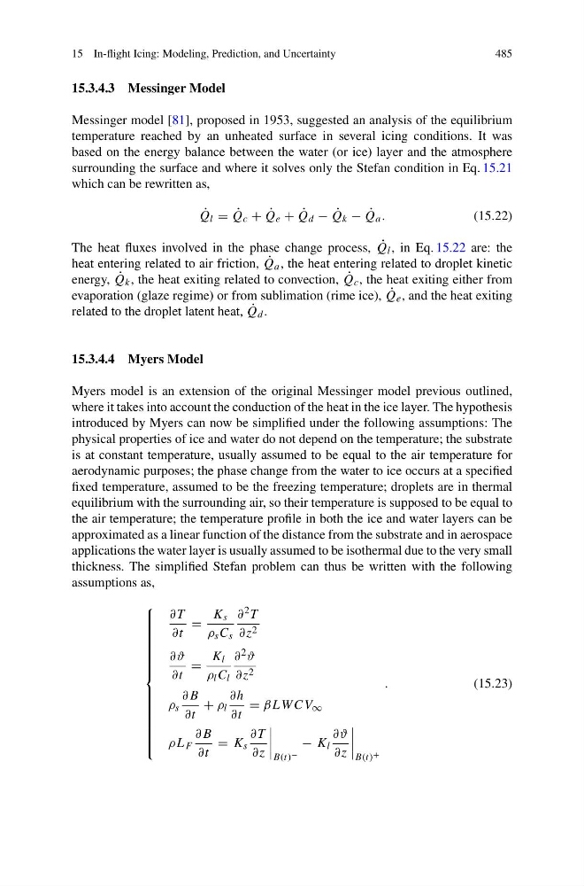
Myers model is an extension of the original Messinger model previous outlined,
where it takes into account the conduction of the heat in the ice layer. The hypothesis
introduced by Myers can now be simplified under the following assumptions: The
physical properties of ice and water do not depend on the temperature; the substrate
is at constant temperature, usually assumed to be equal to the air temperature for
aerodynamic purposes; the phase change from the water to ice occurs at a specified
fixed temperature, assumed to be the freezing temperature; droplets are in thermal
equilibrium with the surrounding air, so their temperature is supposed to be equal to
the air temperature; the temperature profile in both the ice and water layers can be
approximated as a linear function of the distance from the substrate and in aerospace
applications the water layer is usually assumed to be isothermal due to the very small
thickness. The simplified Stefan problem can thus be written with the following
assumptions as,
⎧
⎪ ⎪ ⎪ ⎪ ⎪ ⎪ ⎪ ⎪ ⎪ ⎪ ⎪ ⎪ ⎪ ⎨
⎪ ⎪ ⎪ ⎪ ⎪ ⎪ ⎪ ⎪ ⎪ ⎪ ⎪ ⎪ ⎪ ⎩
∂T
∂t
=
K s
ρ s C s
∂ 2 T
∂z 2
∂ϑ
∂t
=
K l
ρ l C l
∂ 2 ϑ
∂z 2
ρ s
∂B
∂t
+ ρ l
∂h
∂t
= βLW CV ∞
ρL F
∂B
∂t
= K s
∂T
∂z
B(t) −
− K l
∂ϑ
∂z
B(t) +
.
(15.23)
485
15.3.4.3 Messinger Model
Messinger model [81], proposed in 1953, suggested an analysis of the equilibrium
temperature reached by an unheated surface in several icing conditions. It was
based on the energy balance between the water (or ice) layer and the atmosphere
surrounding the surface and where it solves only the Stefan condition in Eq. 15.21
which can be rewritten as,
˙
Q l = ˙
Q c + ˙
Q e + ˙
Q d − ˙
Q k − ˙
Q a .
(15.22)
The heat fluxes involved in the phase change process, ˙
Q l , in Eq. 15.22 are: the
heat entering related to air friction, ˙
Q a , the heat entering related to droplet kinetic
energy, ˙
Q k , the heat exiting related to convection, ˙
Q c , the heat exiting either from
evaporation (glaze regime) or from sublimation (rime ice), ˙
Q e , and the heat exiting
related to the droplet latent heat, ˙
Q d .
15.3.4.4 Myers Model
Myers model is an extension of the original Messinger model previous outlined,
where it takes into account the conduction of the heat in the ice layer. The hypothesis
introduced by Myers can now be simplified under the following assumptions: The
physical properties of ice and water do not depend on the temperature; the substrate
is at constant temperature, usually assumed to be equal to the air temperature for
aerodynamic purposes; the phase change from the water to ice occurs at a specified
fixed temperature, assumed to be the freezing temperature; droplets are in thermal
equilibrium with the surrounding air, so their temperature is supposed to be equal to
the air temperature; the temperature profile in both the ice and water layers can be
approximated as a linear function of the distance from the substrate and in aerospace
applications the water layer is usually assumed to be isothermal due to the very small
thickness. The simplified Stefan problem can thus be written with the following
assumptions as,
⎧
⎪ ⎪ ⎪ ⎪ ⎪ ⎪ ⎪ ⎪ ⎪ ⎪ ⎪ ⎪ ⎪ ⎨
⎪ ⎪ ⎪ ⎪ ⎪ ⎪ ⎪ ⎪ ⎪ ⎪ ⎪ ⎪ ⎪ ⎩
∂T
∂t
=
K s
ρ s C s
∂ 2 T
∂z 2
∂ϑ
∂t
=
K l
ρ l C l
∂ 2 ϑ
∂z 2
ρ s
∂B
∂t
+ ρ l
∂h
∂t
= βLW CV ∞
ρL F
∂B
∂t
= K s
∂T
∂z
B(t) −
− K l
∂ϑ
∂z
B(t) +
.
(15.23)