

484
B. Arizmendi et al.
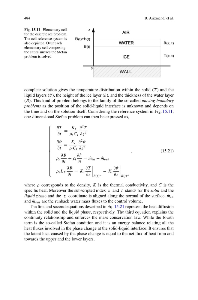
Fig. 15.11 Elementary cell
for the discrete ice problem.
The cell reference system is
also depicted. Over each
elementary cell composing
the entire surface the Stefan
problem is solved
complete solution gives the temperature distribution within the solid (T ) and the
liquid layers (ϑ), the height of the ice layer (h), and the thickness of the water layer
(B). This kind of problem belongs to the family of the so-called moving-boundary
problems as the position of the solid-liquid interface is unknown and depends on
the time and on the solution itself. Considering the reference system in Fig. 15.11,
one-dimensional Stefan problem can then be expressed as,
⎧
⎪ ⎪ ⎪ ⎪ ⎪ ⎪ ⎪ ⎪ ⎪ ⎪ ⎪ ⎪ ⎪ ⎨
⎪ ⎪ ⎪ ⎪ ⎪ ⎪ ⎪ ⎪ ⎪ ⎪ ⎪ ⎪ ⎪ ⎩
∂T
∂t
=
K s
ρ s C s
∂ 2 T
∂z 2
∂ϑ
∂t
=
K l
ρ l C l
∂ 2 ϑ
∂z 2
ρ s
∂B
∂t
+ ρ l
∂h
∂t
= ˙
m in − ˙
m out
ρ s L F
∂B
∂t
= K s
∂T
∂z
B(t) −
− K l
∂ϑ
∂z
B(t) +
,
(15.21)
where ρ corresponds to the density, K is the thermal conductivity, and C is the
specific heat. Moreover the subscripted index s and l stands for the solid and the
liquid phase and the z coordinate is aligned along the normal of the surface. ˙
m in
and ˙
m out are the runback water mass fluxes to the control volume.
The first and second equations described in Eq. 15.21 represent the heat diffusion
within the solid and the liquid phase, respectively. The third equation explains the
continuity relationship and enforces the mass conservation law. While the fourth
term is the so-called Stefan condition and it is an energy balance relating all the
heat fluxes involved in the phase change at the solid-liquid interface. It ensures that
the latent heat caused by the phase change is equal to the net flux of heat from and
towards the upper and the lower layers.
B. Arizmendi et al.
Fig. 15.11 Elementary cell
for the discrete ice problem.
The cell reference system is
also depicted. Over each
elementary cell composing
the entire surface the Stefan
problem is solved
complete solution gives the temperature distribution within the solid (T ) and the
liquid layers (ϑ), the height of the ice layer (h), and the thickness of the water layer
(B). This kind of problem belongs to the family of the so-called moving-boundary
problems as the position of the solid-liquid interface is unknown and depends on
the time and on the solution itself. Considering the reference system in Fig. 15.11,
one-dimensional Stefan problem can then be expressed as,
⎧
⎪ ⎪ ⎪ ⎪ ⎪ ⎪ ⎪ ⎪ ⎪ ⎪ ⎪ ⎪ ⎪ ⎨
⎪ ⎪ ⎪ ⎪ ⎪ ⎪ ⎪ ⎪ ⎪ ⎪ ⎪ ⎪ ⎪ ⎩
∂T
∂t
=
K s
ρ s C s
∂ 2 T
∂z 2
∂ϑ
∂t
=
K l
ρ l C l
∂ 2 ϑ
∂z 2
ρ s
∂B
∂t
+ ρ l
∂h
∂t
= ˙
m in − ˙
m out
ρ s L F
∂B
∂t
= K s
∂T
∂z
B(t) −
− K l
∂ϑ
∂z
B(t) +
,
(15.21)
where ρ corresponds to the density, K is the thermal conductivity, and C is the
specific heat. Moreover the subscripted index s and l stands for the solid and the
liquid phase and the z coordinate is aligned along the normal of the surface. ˙
m in
and ˙
m out are the runback water mass fluxes to the control volume.
The first and second equations described in Eq. 15.21 represent the heat diffusion
within the solid and the liquid phase, respectively. The third equation explains the
continuity relationship and enforces the mass conservation law. While the fourth
term is the so-called Stefan condition and it is an energy balance relating all the
heat fluxes involved in the phase change at the solid-liquid interface. It ensures that
the latent heat caused by the phase change is equal to the net flux of heat from and
towards the upper and the lower layers.