

15 In-flight Icing: Modeling, Prediction, and Uncertainty
481
where two-dimensional flow conditions are modeled, the process evaluates two
additional trajectories, each a small displacement either side of the trajectory. This
is the method used by LEWICE, FENSAP, and PoliMIce.
15.3.3.1 Eulerian and Lagrangian Specifications for Particle Tracking
Although several codes exist for simulating ice accretion, all have been developed
using different methodologies for solving the complex issue of icing, each with
their own strengths and weaknesses. The majority have either used Eulerian or
Lagrangian particle tracking frameworks to model the physics of ice accretion.
FENSAP-ICE solves the particle governing equations using an Eulerian approach
[59], meanwhile PoliMIce [60] and ONERA [58] use a Lagrangian particle tracking
solver to compute the droplet trajectories. In classical field theory the Lagrangian
specification of the field is a way of looking at fluid motion where the observer
follows an individual fluid parcel as it moves through space and time [85]. The
position of particles through time gives the path line of these particles. These fluid
particles have mass, momentum, internal energy, and other properties. Mathematical
laws can then be written for each fluid particle. The Eulerian paradigm of the flow
field is a way of looking at fluid motion that focuses on specific locations in the space
through which the fluid flows as time passes [85]. In the Eulerian specification of a
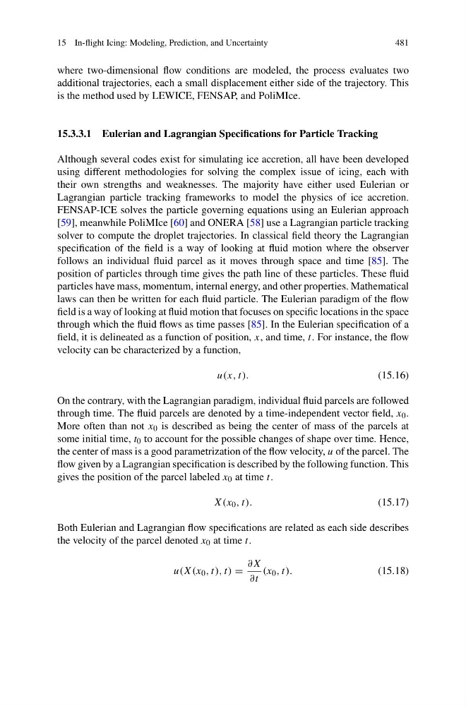
field, it is delineated as a function of position, x, and time, t. For instance, the flow
velocity can be characterized by a function,
u(x, t).
(15.16)
On the contrary, with the Lagrangian paradigm, individual fluid parcels are followed
through time. The fluid parcels are denoted by a time-independent vector field, x 0 .
More often than not x 0 is described as being the center of mass of the parcels at
some initial time, t 0 to account for the possible changes of shape over time. Hence,
the center of mass is a good parametrization of the flow velocity, u of the parcel. The
flow given by a Lagrangian specification is described by the following function. This
gives the position of the parcel labeled x 0 at time t.
X(x 0 , t).
(15.17)
Both Eulerian and Lagrangian flow specifications are related as each side describes
the velocity of the parcel denoted x 0 at time t.
u(X(x 0 , t), t) =
∂X
∂t
(x 0 , t).
(15.18)
481
where two-dimensional flow conditions are modeled, the process evaluates two
additional trajectories, each a small displacement either side of the trajectory. This
is the method used by LEWICE, FENSAP, and PoliMIce.
15.3.3.1 Eulerian and Lagrangian Specifications for Particle Tracking
Although several codes exist for simulating ice accretion, all have been developed
using different methodologies for solving the complex issue of icing, each with
their own strengths and weaknesses. The majority have either used Eulerian or
Lagrangian particle tracking frameworks to model the physics of ice accretion.
FENSAP-ICE solves the particle governing equations using an Eulerian approach
[59], meanwhile PoliMIce [60] and ONERA [58] use a Lagrangian particle tracking
solver to compute the droplet trajectories. In classical field theory the Lagrangian
specification of the field is a way of looking at fluid motion where the observer
follows an individual fluid parcel as it moves through space and time [85]. The
position of particles through time gives the path line of these particles. These fluid
particles have mass, momentum, internal energy, and other properties. Mathematical
laws can then be written for each fluid particle. The Eulerian paradigm of the flow
field is a way of looking at fluid motion that focuses on specific locations in the space
through which the fluid flows as time passes [85]. In the Eulerian specification of a
field, it is delineated as a function of position, x, and time, t. For instance, the flow
velocity can be characterized by a function,
u(x, t).
(15.16)
On the contrary, with the Lagrangian paradigm, individual fluid parcels are followed
through time. The fluid parcels are denoted by a time-independent vector field, x 0 .
More often than not x 0 is described as being the center of mass of the parcels at
some initial time, t 0 to account for the possible changes of shape over time. Hence,
the center of mass is a good parametrization of the flow velocity, u of the parcel. The
flow given by a Lagrangian specification is described by the following function. This
gives the position of the parcel labeled x 0 at time t.
X(x 0 , t).
(15.17)
Both Eulerian and Lagrangian flow specifications are related as each side describes
the velocity of the parcel denoted x 0 at time t.
u(X(x 0 , t), t) =
∂X
∂t
(x 0 , t).
(15.18)