

9 Multilevel Optimisation
313
1.6
1.8
2
2.2
2.4
2.6
2.8
x
1.6
1.8
2
2.2
2.4
2.6
2.8
y
Linear Bilevel Optimisation Example
A
D
C
B
-20
-19
-18
-17
-16
-15
-14
-13
-12
-11
-10
x-8 y
-x-y<=-4
-x+y<=0
3x+y<=10
-3x+2y>=-3
Feasible Area
min f(y) = y
min F(x,y)
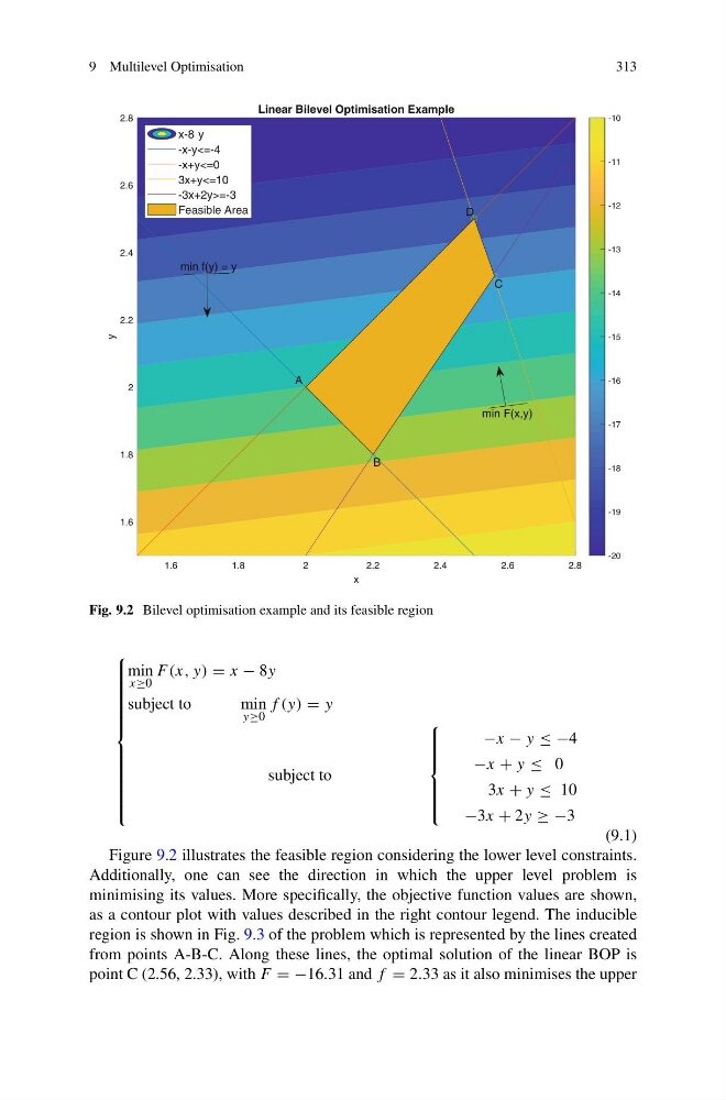
Fig. 9.2 Bilevel optimisation example and its feasible region
⎧
⎪ ⎪ ⎪ ⎪ ⎪ ⎪ ⎪ ⎪ ⎪ ⎪ ⎪ ⎨
⎪ ⎪ ⎪ ⎪ ⎪ ⎪ ⎪ ⎪ ⎪ ⎪ ⎪ ⎩
min
x≥0
F (x, y) = x − 8y
subject to
min
y≥0
f (y) = y
subject to
⎧
⎪ ⎪ ⎪ ⎪ ⎨
⎪ ⎪ ⎪ ⎪ ⎩
−x − y ≤ −4
−x + y ≤ 0
3x + y ≤ 10
−3x + 2y ≥ −3
(9.1)
Figure 9.2 illustrates the feasible region considering the lower level constraints.
Additionally, one can see the direction in which the upper level problem is
minimising its values. More specifically, the objective function values are shown,
as a contour plot with values described in the right contour legend. The inducible
region is shown in Fig. 9.3 of the problem which is represented by the lines created
from points A-B-C. Along these lines, the optimal solution of the linear BOP is
point C (2.56, 2.33), with F = −16.31 and f = 2.33 as it also minimises the upper
313
1.6
1.8
2
2.2
2.4
2.6
2.8
x
1.6
1.8
2
2.2
2.4
2.6
2.8
y
Linear Bilevel Optimisation Example
A
D
C
B
-20
-19
-18
-17
-16
-15
-14
-13
-12
-11
-10
x-8 y
-x-y<=-4
-x+y<=0
3x+y<=10
-3x+2y>=-3
Feasible Area
min f(y) = y
min F(x,y)
Fig. 9.2 Bilevel optimisation example and its feasible region
⎧
⎪ ⎪ ⎪ ⎪ ⎪ ⎪ ⎪ ⎪ ⎪ ⎪ ⎪ ⎨
⎪ ⎪ ⎪ ⎪ ⎪ ⎪ ⎪ ⎪ ⎪ ⎪ ⎪ ⎩
min
x≥0
F (x, y) = x − 8y
subject to
min
y≥0
f (y) = y
subject to
⎧
⎪ ⎪ ⎪ ⎪ ⎨
⎪ ⎪ ⎪ ⎪ ⎩
−x − y ≤ −4
−x + y ≤ 0
3x + y ≤ 10
−3x + 2y ≥ −3
(9.1)
Figure 9.2 illustrates the feasible region considering the lower level constraints.
Additionally, one can see the direction in which the upper level problem is
minimising its values. More specifically, the objective function values are shown,
as a contour plot with values described in the right contour legend. The inducible
region is shown in Fig. 9.3 of the problem which is represented by the lines created
from points A-B-C. Along these lines, the optimal solution of the linear BOP is
point C (2.56, 2.33), with F = −16.31 and f = 2.33 as it also minimises the upper