

290
D. Irawan and B. Naujoks
of the last ranked front to a reference line instead of the distances to its neighbor.
So instead of comparing distances of K − μ individuals to all other 2μ − 1 points
in each dimension, NSGA-III only needs to calculate distances between the K − μ
individuals to
M+p−1
p
reference lines.
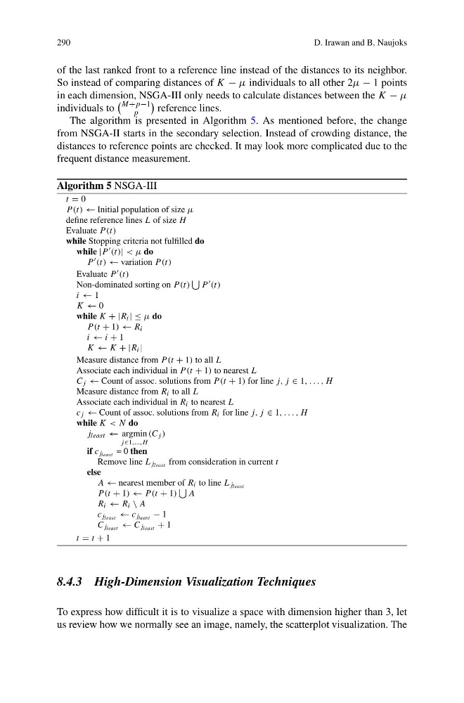
The algorithm is presented in Algorithm 5. As mentioned before, the change
from NSGA-II starts in the secondary selection. Instead of crowding distance, the
distances to reference points are checked. It may look more complicated due to the
frequent distance measurement.
Algorithm 5 NSGA-III
t = 0
P (t) ← Initial population of size μ
define reference lines L of size H
Evaluate P (t)
while Stopping criteria not fulfilled do
while |P (t)| < μ do
P (t) ← variation P (t)
Evaluate P (t)
Non-dominated sorting on P (t)
P (t)
i ← 1
K ← 0
while K + |R i | ≤ μ do
P (t + 1) ← R i
i ← i + 1
K ← K + |R i |
Measure distance from P (t + 1) to all L
Associate each individual in P (t + 1) to nearest L
C j ← Count of assoc. solutions from P (t + 1) for line j, j ∈ 1, . . . , H
Measure distance from R i to all L
Associate each individual in R i to nearest L
c j ← Count of assoc. solutions from R i for line j, j ∈ 1, . . . , H
while K < N do
j least ← argmin
j ∈1,...,H
(C j )
if c j least = 0 then
Remove line L j least from consideration in current t
else
A ← nearest member of R i to line L j least
P (t + 1) ← P (t + 1)
A
R i ← R i \ A
c j least ← c j least − 1
C j least ← C j least + 1
t = t + 1
8.4.3 High-Dimension Visualization Techniques
To express how difficult it is to visualize a space with dimension higher than 3, let
us review how we normally see an image, namely, the scatterplot visualization. The
D. Irawan and B. Naujoks
of the last ranked front to a reference line instead of the distances to its neighbor.
So instead of comparing distances of K − μ individuals to all other 2μ − 1 points
in each dimension, NSGA-III only needs to calculate distances between the K − μ
individuals to
M+p−1
p
reference lines.
The algorithm is presented in Algorithm 5. As mentioned before, the change
from NSGA-II starts in the secondary selection. Instead of crowding distance, the
distances to reference points are checked. It may look more complicated due to the
frequent distance measurement.
Algorithm 5 NSGA-III
t = 0
P (t) ← Initial population of size μ
define reference lines L of size H
Evaluate P (t)
while Stopping criteria not fulfilled do
while |P (t)| < μ do
P (t) ← variation P (t)
Evaluate P (t)
Non-dominated sorting on P (t)
P (t)
i ← 1
K ← 0
while K + |R i | ≤ μ do
P (t + 1) ← R i
i ← i + 1
K ← K + |R i |
Measure distance from P (t + 1) to all L
Associate each individual in P (t + 1) to nearest L
C j ← Count of assoc. solutions from P (t + 1) for line j, j ∈ 1, . . . , H
Measure distance from R i to all L
Associate each individual in R i to nearest L
c j ← Count of assoc. solutions from R i for line j, j ∈ 1, . . . , H
while K < N do
j least ← argmin
j ∈1,...,H
(C j )
if c j least = 0 then
Remove line L j least from consideration in current t
else
A ← nearest member of R i to line L j least
P (t + 1) ← P (t + 1)
A
R i ← R i \ A
c j least ← c j least − 1
C j least ← C j least + 1
t = t + 1
8.4.3 High-Dimension Visualization Techniques
To express how difficult it is to visualize a space with dimension higher than 3, let
us review how we normally see an image, namely, the scatterplot visualization. The