

8 An Introduction to Many-Objective Evolutionary Optimization
289
8.4.2.2 NSGA-III
NSGA-III by Deb et al. [11] is a recent addition to the library of MOEA algorithms.
As the name suggests, it has a similarity with NSGA-II. In fact, NSGA-II is also
invented by Deb and his colleagues [12].
As a note, originally, NSGA-III can work well only on many-objective problems.
However, Seada [37] together with Deb modified the algorithm to work on lower
dimensions in their subsequent publication on unified NSGA-III (UNSGA-III). This
section, however, only describes the original NSGA-III.
NSGA-III starts with recombination and mutation to generate offspring P , then
uses the same non-dominated sorting as in NSGA-II and SMS-EMOA, but that
is where the similarity ends. For the secondary selection operator, NSGA-III is
more akin to MOEA/D: it uses reference points. While in MOEA/D we use one
reference point with multiple search directions based on the weight vectors (i.e., for
each weight, one optimization loop is conducted), NSGA-III opts to use multiple
reference points representing different weights of the objectives (i.e., in a single
optimization loop, all weights are considered).
The number and locations of reference points can vary depending on preference,
Deb and Jain [11] showed that the method can work with both structured and
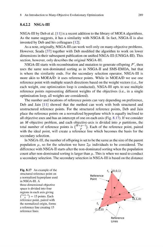
unstructured reference points. For the structured reference points, Deb and Jain
place the reference points on a normalized hyperplane which is equally inclined to
all objective axes and has an intercept of one on each axis (Fig. 8.17). If we consider
an M-objective problem, and each objective-axis is divided into p partitions, the
total number of reference points is
M+p−1
p
. Each of the reference point, paired
with the ideal point, will create a reference line which becomes the basis for the
secondary selection.
In NSGA-III, the number of offspring is set to be the same as the size of the parent
population μ, so for the selection we have 2μ individuals to be considered. The
difference with NSGA-II starts after the non-dominated sorting when the population
count after non-dominated sorting is larger than μ. This is when we need to conduct
a secondary selection. The secondary selection in NSGA-III is based on the distance
Fig. 8.17 An example of the
structured reference point on
a normalized hyperplane used
in NSGA-III. A
three-dimensional objective
space is divided into four
regions in each axis giving
3+4−1
4
= 15 points. Each
reference point, paired with
the normalized origin, forms
a reference line creating 15
reference lines
289
8.4.2.2 NSGA-III
NSGA-III by Deb et al. [11] is a recent addition to the library of MOEA algorithms.
As the name suggests, it has a similarity with NSGA-II. In fact, NSGA-II is also
invented by Deb and his colleagues [12].
As a note, originally, NSGA-III can work well only on many-objective problems.
However, Seada [37] together with Deb modified the algorithm to work on lower
dimensions in their subsequent publication on unified NSGA-III (UNSGA-III). This
section, however, only describes the original NSGA-III.
NSGA-III starts with recombination and mutation to generate offspring P , then
uses the same non-dominated sorting as in NSGA-II and SMS-EMOA, but that
is where the similarity ends. For the secondary selection operator, NSGA-III is
more akin to MOEA/D: it uses reference points. While in MOEA/D we use one
reference point with multiple search directions based on the weight vectors (i.e., for
each weight, one optimization loop is conducted), NSGA-III opts to use multiple
reference points representing different weights of the objectives (i.e., in a single
optimization loop, all weights are considered).
The number and locations of reference points can vary depending on preference,
Deb and Jain [11] showed that the method can work with both structured and
unstructured reference points. For the structured reference points, Deb and Jain
place the reference points on a normalized hyperplane which is equally inclined to
all objective axes and has an intercept of one on each axis (Fig. 8.17). If we consider
an M-objective problem, and each objective-axis is divided into p partitions, the
total number of reference points is
M+p−1
p
. Each of the reference point, paired
with the ideal point, will create a reference line which becomes the basis for the
secondary selection.
In NSGA-III, the number of offspring is set to be the same as the size of the parent
population μ, so for the selection we have 2μ individuals to be considered. The
difference with NSGA-II starts after the non-dominated sorting when the population
count after non-dominated sorting is larger than μ. This is when we need to conduct
a secondary selection. The secondary selection in NSGA-III is based on the distance
Fig. 8.17 An example of the
structured reference point on
a normalized hyperplane used
in NSGA-III. A
three-dimensional objective
space is divided into four
regions in each axis giving
3+4−1
4
= 15 points. Each
reference point, paired with
the normalized origin, forms
a reference line creating 15
reference lines