

288
D. Irawan and B. Naujoks
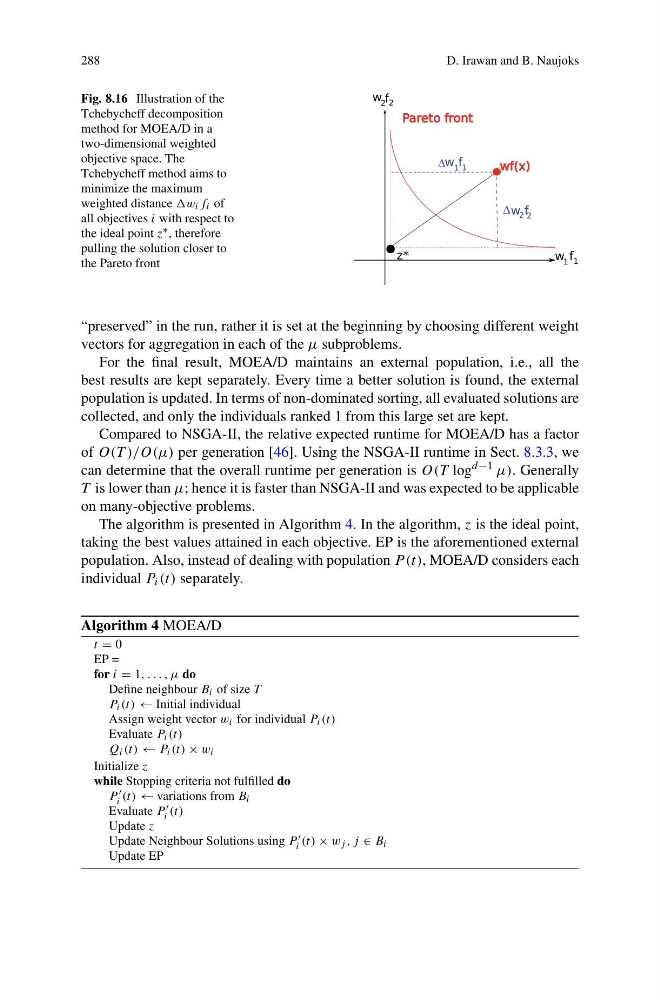
Fig. 8.16 Illustration of the
Tchebycheff decomposition
method for MOEA/D in a
two-dimensional weighted
objective space. The
Tchebycheff method aims to
minimize the maximum
weighted distance w i f i of
all objectives i with respect to
the ideal point z ∗ , therefore
pulling the solution closer to
the Pareto front
“preserved” in the run, rather it is set at the beginning by choosing different weight
vectors for aggregation in each of the μ subproblems.
For the final result, MOEA/D maintains an external population, i.e., all the
best results are kept separately. Every time a better solution is found, the external
population is updated. In terms of non-dominated sorting, all evaluated solutions are
collected, and only the individuals ranked 1 from this large set are kept.
Compared to NSGA-II, the relative expected runtime for MOEA/D has a factor
of O(T )/O(μ) per generation [46]. Using the NSGA-II runtime in Sect. 8.3.3, we
can determine that the overall runtime per generation is O(T log
d−1 μ). Generally
T is lower than μ; hence it is faster than NSGA-II and was expected to be applicable
on many-objective problems.
The algorithm is presented in Algorithm 4. In the algorithm, z is the ideal point,
taking the best values attained in each objective. EP is the aforementioned external
population. Also, instead of dealing with population P (t), MOEA/D considers each
individual P i (t) separately.
Algorithm 4 MOEA/D
t = 0
EP =
for i = 1, . . . , μ do
Define neighbour B i of size T
P i (t) ← Initial individual
Assign weight vector w i for individual P i (t)
Evaluate P i (t)
Q i (t) ← P i (t) × w i
Initialize z
while Stopping criteria not fulfilled do
P
i (t) ← variations from B i
Evaluate P
i (t)
Update z
Update Neighbour Solutions using P
i (t) × w j , j ∈ B i
Update EP
D. Irawan and B. Naujoks
Fig. 8.16 Illustration of the
Tchebycheff decomposition
method for MOEA/D in a
two-dimensional weighted
objective space. The
Tchebycheff method aims to
minimize the maximum
weighted distance w i f i of
all objectives i with respect to
the ideal point z ∗ , therefore
pulling the solution closer to
the Pareto front
“preserved” in the run, rather it is set at the beginning by choosing different weight
vectors for aggregation in each of the μ subproblems.
For the final result, MOEA/D maintains an external population, i.e., all the
best results are kept separately. Every time a better solution is found, the external
population is updated. In terms of non-dominated sorting, all evaluated solutions are
collected, and only the individuals ranked 1 from this large set are kept.
Compared to NSGA-II, the relative expected runtime for MOEA/D has a factor
of O(T )/O(μ) per generation [46]. Using the NSGA-II runtime in Sect. 8.3.3, we
can determine that the overall runtime per generation is O(T log
d−1 μ). Generally
T is lower than μ; hence it is faster than NSGA-II and was expected to be applicable
on many-objective problems.
The algorithm is presented in Algorithm 4. In the algorithm, z is the ideal point,
taking the best values attained in each objective. EP is the aforementioned external
population. Also, instead of dealing with population P (t), MOEA/D considers each
individual P i (t) separately.
Algorithm 4 MOEA/D
t = 0
EP =
for i = 1, . . . , μ do
Define neighbour B i of size T
P i (t) ← Initial individual
Assign weight vector w i for individual P i (t)
Evaluate P i (t)
Q i (t) ← P i (t) × w i
Initialize z
while Stopping criteria not fulfilled do
P
i (t) ← variations from B i
Evaluate P
i (t)
Update z
Update Neighbour Solutions using P
i (t) × w j , j ∈ B i
Update EP