

272
D. Irawan and B. Naujoks
9
8
7
6
5
4
3
2
1
0
0
2
4
6
8
1 0
1 2
1 4
1 6
f
2
f 1
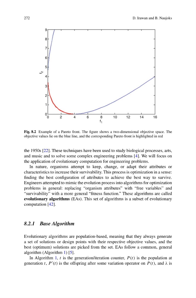
Fig. 8.2 Example of a Pareto front. The figure shows a two-dimensional objective space. The
objective values lie on the blue line, and the corresponding Pareto front is highlighted in red
the 1950s [22]. These techniques have been used to study biological processes, arts,
and music and to solve some complex engineering problems [4]. We will focus on
the application of evolutionary computation for engineering problems.
In nature, organisms attempt to keep, change, or adapt their attributes or
characteristics to increase their survivability. This process is optimization in a sense:
finding the best configuration of attributes to achieve the best way to survive.
Engineers attempted to mimic the evolution process into algorithms for optimization
problems in general: replacing “organism attributes” with “free variables” and
“survivability” with a more general “fitness function.” These algorithms are called
evolutionary algorithms (EAs). This set of algorithms is a subset of evolutionary
computation [42].
8.2.1 Base Algorithm
Evolutionary algorithms are population-based, meaning that they always generate
a set of solutions or design points with their respective objective values, and the
best (optimum) solutions are picked from the set. EAs follow a common, general
algorithm (Algorithm 1) [5].
In Algorithm 1, t is the generation/iteration counter, P (t) is the population at
generation t, P (t) is the offspring after some variation operator on P (t), and λ is
D. Irawan and B. Naujoks
9
8
7
6
5
4
3
2
1
0
0
2
4
6
8
1 0
1 2
1 4
1 6
f
2
f 1
Fig. 8.2 Example of a Pareto front. The figure shows a two-dimensional objective space. The
objective values lie on the blue line, and the corresponding Pareto front is highlighted in red
the 1950s [22]. These techniques have been used to study biological processes, arts,
and music and to solve some complex engineering problems [4]. We will focus on
the application of evolutionary computation for engineering problems.
In nature, organisms attempt to keep, change, or adapt their attributes or
characteristics to increase their survivability. This process is optimization in a sense:
finding the best configuration of attributes to achieve the best way to survive.
Engineers attempted to mimic the evolution process into algorithms for optimization
problems in general: replacing “organism attributes” with “free variables” and
“survivability” with a more general “fitness function.” These algorithms are called
evolutionary algorithms (EAs). This set of algorithms is a subset of evolutionary
computation [42].
8.2.1 Base Algorithm
Evolutionary algorithms are population-based, meaning that they always generate
a set of solutions or design points with their respective objective values, and the
best (optimum) solutions are picked from the set. EAs follow a common, general
algorithm (Algorithm 1) [5].
In Algorithm 1, t is the generation/iteration counter, P (t) is the population at
generation t, P (t) is the offspring after some variation operator on P (t), and λ is