

8 An Introduction to Many-Objective Evolutionary Optimization
271
9
8
7
6
5
4
3
2
1
0
0
2
4
6
8
1 0
1 2
1 4
1 6
f 1
f
2
Does not dominate each other
A dominate B
A
B
X1
X2
X3
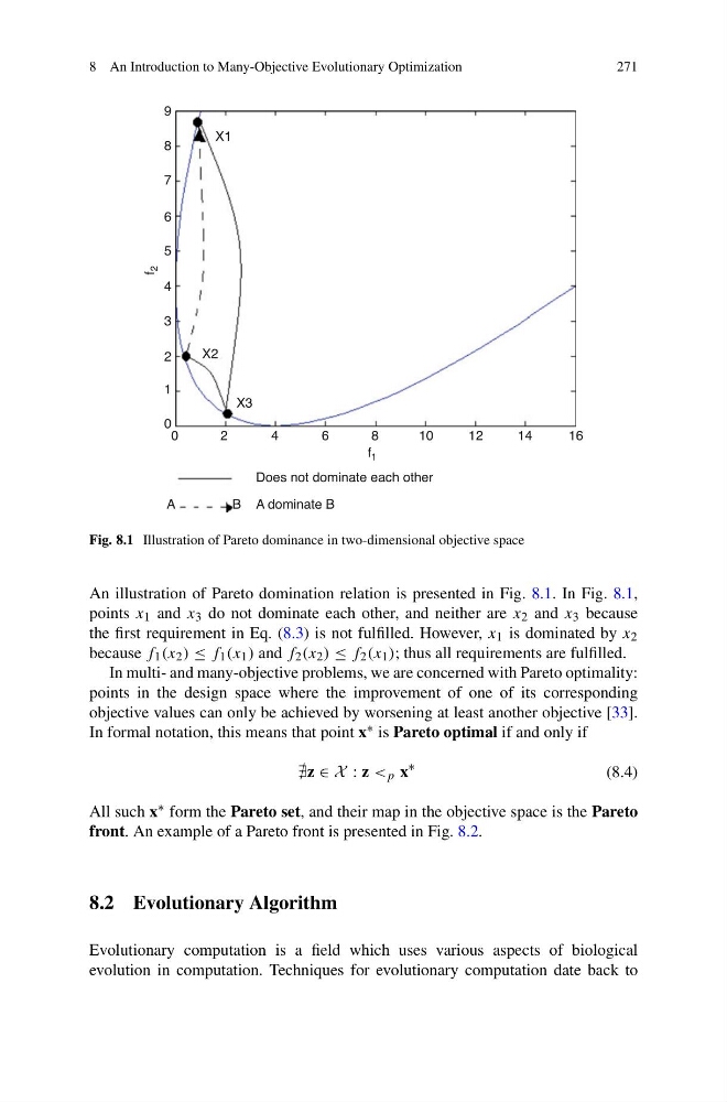
Fig. 8.1 Illustration of Pareto dominance in two-dimensional objective space
An illustration of Pareto domination relation is presented in Fig. 8.1. In Fig. 8.1,
points x 1 and x 3 do not dominate each other, and neither are x 2 and x 3 because
the first requirement in Eq. (8.3) is not fulfilled. However, x 1 is dominated by x 2
because f 1 (x 2 ) ≤ f 1 (x 1 ) and f 2 (x 2 ) ≤ f 2 (x 1 ); thus all requirements are fulfilled.
In multi- and many-objective problems, we are concerned with Pareto optimality:
points in the design space where the improvement of one of its corresponding
objective values can only be achieved by worsening at least another objective [33].
In formal notation, this means that point x ∗ is Pareto optimal if and only if
z ∈ X : z < p x
∗
(8.4)
All such x ∗ form the Pareto set, and their map in the objective space is the Pareto
front. An example of a Pareto front is presented in Fig. 8.2.
8.2 Evolutionary Algorithm
Evolutionary computation is a field which uses various aspects of biological
evolution in computation. Techniques for evolutionary computation date back to
271
9
8
7
6
5
4
3
2
1
0
0
2
4
6
8
1 0
1 2
1 4
1 6
f 1
f
2
Does not dominate each other
A dominate B
A
B
X1
X2
X3
Fig. 8.1 Illustration of Pareto dominance in two-dimensional objective space
An illustration of Pareto domination relation is presented in Fig. 8.1. In Fig. 8.1,
points x 1 and x 3 do not dominate each other, and neither are x 2 and x 3 because
the first requirement in Eq. (8.3) is not fulfilled. However, x 1 is dominated by x 2
because f 1 (x 2 ) ≤ f 1 (x 1 ) and f 2 (x 2 ) ≤ f 2 (x 1 ); thus all requirements are fulfilled.
In multi- and many-objective problems, we are concerned with Pareto optimality:
points in the design space where the improvement of one of its corresponding
objective values can only be achieved by worsening at least another objective [33].
In formal notation, this means that point x ∗ is Pareto optimal if and only if
z ∈ X : z < p x
∗
(8.4)
All such x ∗ form the Pareto set, and their map in the objective space is the Pareto
front. An example of a Pareto front is presented in Fig. 8.2.
8.2 Evolutionary Algorithm
Evolutionary computation is a field which uses various aspects of biological
evolution in computation. Techniques for evolutionary computation date back to