

270
D. Irawan and B. Naujoks
minimize
x
f : X ⊂ R
n
− → Y ⊂ R,
subject to g(x) ≤ 0
∀x ∈ X
h(x) = 0
∀x ∈ X
(8.1)
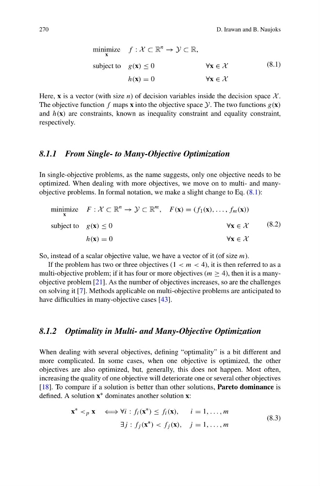
Here, x is a vector (with size n) of decision variables inside the decision space X .
The objective function f maps x into the objective space Y. The two functions g(x)
and h(x) are constraints, known as inequality constraint and equality constraint,
respectively.
8.1.1 From Single- to Many-Objective Optimization
In single-objective problems, as the name suggests, only one objective needs to be
optimized. When dealing with more objectives, we move on to multi- and manyobjective problems. In formal notation, we make a slight change to Eq. (8.1):
minimize
x
F : X ⊂ R
n
− → Y ⊂ R
m , F(x) = (f 1 (x), . . . , f m (x))
subject to g(x) ≤ 0
∀x ∈ X
h(x) = 0
∀x ∈ X
(8.2)
So, instead of a scalar objective value, we have a vector of it (of size m).
If the problem has two or three objectives (1 < m < 4), it is then referred to as a
multi-objective problem; if it has four or more objectives (m ≥ 4), then it is a manyobjective problem [21]. As the number of objectives increases, so are the challenges
on solving it [7]. Methods applicable on multi-objective problems are anticipated to
have difficulties in many-objective cases [43].
8.1.2 Optimality in Multi- and Many-Objective Optimization
When dealing with several objectives, defining “optimality” is a bit different and
more complicated. In some cases, when one objective is optimized, the other
objectives are also optimized, but, generally, this does not happen. Most often,
increasing the quality of one objective will deteriorate one or several other objectives
[18]. To compare if a solution is better than other solutions, Pareto dominance is
defined. A solution x ∗ dominates another solution x:
x
∗ < p x ⇐⇒ ∀i : f i (x
∗ ) ≤ f i (x),
i = 1, . . . , m
∃j : f j (x
∗ ) < f j (x), j = 1, . . . , m
(8.3)
D. Irawan and B. Naujoks
minimize
x
f : X ⊂ R
n
− → Y ⊂ R,
subject to g(x) ≤ 0
∀x ∈ X
h(x) = 0
∀x ∈ X
(8.1)
Here, x is a vector (with size n) of decision variables inside the decision space X .
The objective function f maps x into the objective space Y. The two functions g(x)
and h(x) are constraints, known as inequality constraint and equality constraint,
respectively.
8.1.1 From Single- to Many-Objective Optimization
In single-objective problems, as the name suggests, only one objective needs to be
optimized. When dealing with more objectives, we move on to multi- and manyobjective problems. In formal notation, we make a slight change to Eq. (8.1):
minimize
x
F : X ⊂ R
n
− → Y ⊂ R
m , F(x) = (f 1 (x), . . . , f m (x))
subject to g(x) ≤ 0
∀x ∈ X
h(x) = 0
∀x ∈ X
(8.2)
So, instead of a scalar objective value, we have a vector of it (of size m).
If the problem has two or three objectives (1 < m < 4), it is then referred to as a
multi-objective problem; if it has four or more objectives (m ≥ 4), then it is a manyobjective problem [21]. As the number of objectives increases, so are the challenges
on solving it [7]. Methods applicable on multi-objective problems are anticipated to
have difficulties in many-objective cases [43].
8.1.2 Optimality in Multi- and Many-Objective Optimization
When dealing with several objectives, defining “optimality” is a bit different and
more complicated. In some cases, when one objective is optimized, the other
objectives are also optimized, but, generally, this does not happen. Most often,
increasing the quality of one objective will deteriorate one or several other objectives
[18]. To compare if a solution is better than other solutions, Pareto dominance is
defined. A solution x ∗ dominates another solution x:
x
∗ < p x ⇐⇒ ∀i : f i (x
∗ ) ≤ f i (x),
i = 1, . . . , m
∃j : f j (x
∗ ) < f j (x), j = 1, . . . , m
(8.3)