

1 Introduction to Spectral Methods for Uncertainty Quantification
21
U(x, ξ ) =
P
s=0
u s (x)Ψ n (ξ ).
(1.18)
The N -dimensional polynomials Ψ s are generated from the combination of
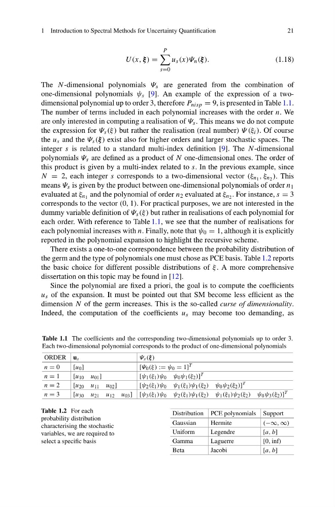
one-dimensional polynomials ψ s [9]. An example of the expression of a twodimensional polynomial up to order 3, therefore P nisp = 9, is presented in Table 1.1.
The number of terms included in each polynomial increases with the order n. We
are only interested in computing a realisation of Ψ s . This means we do not compute
the expression for Ψ s (ξ ) but rather the realisation (real number) Ψ (ξ i ). Of course
the u s and the Ψ s (ξ ) exist also for higher orders and larger stochastic spaces. The
integer s is related to a standard multi-index definition [9]. The N-dimensional
polynomials Ψ s are defined as a product of N one-dimensional ones. The order of
this product is given by a multi-index related to s. In the previous example, since
N = 2, each integer s corresponds to a two-dimensional vector (ξ n 1 , ξ n 2 ). This
means Ψ s is given by the product between one-dimensional polynomials of order n 1
evaluated at ξ n 1 and the polynomial of order n 2 evaluated at ξ n 2 . For instance, s = 3
corresponds to the vector (0, 1). For practical purposes, we are not interested in the
dummy variable definition of Ψ s (ξ ) but rather in realisations of each polynomial for
each order. With reference to Table 1.1, we see that the number of realisations for
each polynomial increases with n. Finally, note that ψ 0 = 1, although it is explicitly
reported in the polynomial expansion to highlight the recursive scheme.
There exists a one-to-one correspondence between the probability distribution of
the germ and the type of polynomials one must chose as PCE basis. Table 1.2 reports
the basic choice for different possible distributions of ξ . A more comprehensive
dissertation on this topic may be found in [12].
Since the polynomial are fixed a priori, the goal is to compute the coefficients
u s of the expansion. It must be pointed out that SM become less efficient as the
dimension N of the germ increases. This is the so-called curse of dimensionality.
Indeed, the computation of the coefficients u s may become too demanding, as
Table 1.1 The coefficients and the corresponding two-dimensional polynomials up to order 3.
Each two-dimensional polynomial corresponds to the product of one-dimensional polynomials
ORDER u s
Ψ s (ξ )
n = 0
[u 0 ]
[Ψ 0 (ξ ) := ψ 0 = 1] T
n = 1
[u 10 u 01 ]
[ψ 1 (ξ 1 )ψ 0 ψ 0 ψ 1 (ξ 2 )] T
n = 2
[u 20 u 11 u 02 ]
[ψ 2 (ξ 1 )ψ 0 ψ 1 (ξ 1 )ψ 1 (ξ 2 ) ψ 0 ψ 2 (ξ 2 )] T
n = 3
[u 30 u 21 u 12 u 03 ] [ψ 3 (ξ 1 )ψ 0 ψ 2 (ξ 1 )ψ 1 (ξ 2 ) ψ 1 (ξ 1 )ψ 2 (ξ 2 ) ψ 0 ψ 3 (ξ 2 )] T
Table 1.2 For each
probability distribution
characterising the stochastic
variables, we are required to
select a specific basis
Distribution PCE polynomials Support
Gaussian
Hermite
(−∞, ∞)
Uniform
Legendre
[a, b]
Gamma
Laguerre
[0, inf)
Beta
Jacobi
[a, b]
21
U(x, ξ ) =
P
s=0
u s (x)Ψ n (ξ ).
(1.18)
The N -dimensional polynomials Ψ s are generated from the combination of
one-dimensional polynomials ψ s [9]. An example of the expression of a twodimensional polynomial up to order 3, therefore P nisp = 9, is presented in Table 1.1.
The number of terms included in each polynomial increases with the order n. We
are only interested in computing a realisation of Ψ s . This means we do not compute
the expression for Ψ s (ξ ) but rather the realisation (real number) Ψ (ξ i ). Of course
the u s and the Ψ s (ξ ) exist also for higher orders and larger stochastic spaces. The
integer s is related to a standard multi-index definition [9]. The N-dimensional
polynomials Ψ s are defined as a product of N one-dimensional ones. The order of
this product is given by a multi-index related to s. In the previous example, since
N = 2, each integer s corresponds to a two-dimensional vector (ξ n 1 , ξ n 2 ). This
means Ψ s is given by the product between one-dimensional polynomials of order n 1
evaluated at ξ n 1 and the polynomial of order n 2 evaluated at ξ n 2 . For instance, s = 3
corresponds to the vector (0, 1). For practical purposes, we are not interested in the
dummy variable definition of Ψ s (ξ ) but rather in realisations of each polynomial for
each order. With reference to Table 1.1, we see that the number of realisations for
each polynomial increases with n. Finally, note that ψ 0 = 1, although it is explicitly
reported in the polynomial expansion to highlight the recursive scheme.
There exists a one-to-one correspondence between the probability distribution of
the germ and the type of polynomials one must chose as PCE basis. Table 1.2 reports
the basic choice for different possible distributions of ξ . A more comprehensive
dissertation on this topic may be found in [12].
Since the polynomial are fixed a priori, the goal is to compute the coefficients
u s of the expansion. It must be pointed out that SM become less efficient as the
dimension N of the germ increases. This is the so-called curse of dimensionality.
Indeed, the computation of the coefficients u s may become too demanding, as
Table 1.1 The coefficients and the corresponding two-dimensional polynomials up to order 3.
Each two-dimensional polynomial corresponds to the product of one-dimensional polynomials
ORDER u s
Ψ s (ξ )
n = 0
[u 0 ]
[Ψ 0 (ξ ) := ψ 0 = 1] T
n = 1
[u 10 u 01 ]
[ψ 1 (ξ 1 )ψ 0 ψ 0 ψ 1 (ξ 2 )] T
n = 2
[u 20 u 11 u 02 ]
[ψ 2 (ξ 1 )ψ 0 ψ 1 (ξ 1 )ψ 1 (ξ 2 ) ψ 0 ψ 2 (ξ 2 )] T
n = 3
[u 30 u 21 u 12 u 03 ] [ψ 3 (ξ 1 )ψ 0 ψ 2 (ξ 1 )ψ 1 (ξ 2 ) ψ 1 (ξ 1 )ψ 2 (ξ 2 ) ψ 0 ψ 3 (ξ 2 )] T
Table 1.2 For each
probability distribution
characterising the stochastic
variables, we are required to
select a specific basis
Distribution PCE polynomials Support
Gaussian
Hermite
(−∞, ∞)
Uniform
Legendre
[a, b]
Gamma
Laguerre
[0, inf)
Beta
Jacobi
[a, b]