

22
J. F. Reis et al.
the number of realisations required to determine these deterministic coefficients
increases exponentially, with the dimension of the germ. Moreover, the construction
of N-dimensional polynomials gets more complex for higher order polynomials.
This means that the computation complexity also increases with N 0 . Therefore, we
need to find a balance between the accuracy and the computational cost.
There are several approaches to construct the PCE Eq. (1.17). In the following
sections, we will present two different methods: Non-Intrusive Spectral Projection
(NISP) and Galerkin methods.
As for the MC approach, NISP methods rely on deterministic evaluations of the
considered model, to compute the PCE coefficients and to obtain the surrogate. Once
the coefficients are available, the statistics of the output can be directly retrieved by
established expressions. Indeed, there exist formulae that relate the coefficients to
the statistics of the QoI. For instance, the coefficient u 0 is equal to the mean of the
surrogate output.
1.6.2 Non-Intrusive Spectral Projection Methods
The goal of the chapter is to present clever techniques to retrieve certain information
about a stochastic process. In general one could think of a model as a surjective
mapping between the space of the parametrised input parameters and the QoI.
Non-intrusive spectral projection methods rely on the construction of a spectral
expansion of the stochastic process. The surrogate approximates the behaviour of
the original model in the sense that it is able to dictate a surjective mapping, up to a
certain level of accuracy, between the stochastic input space and the output domain.
The input parameters can be thus linked to the output through a functional relation.
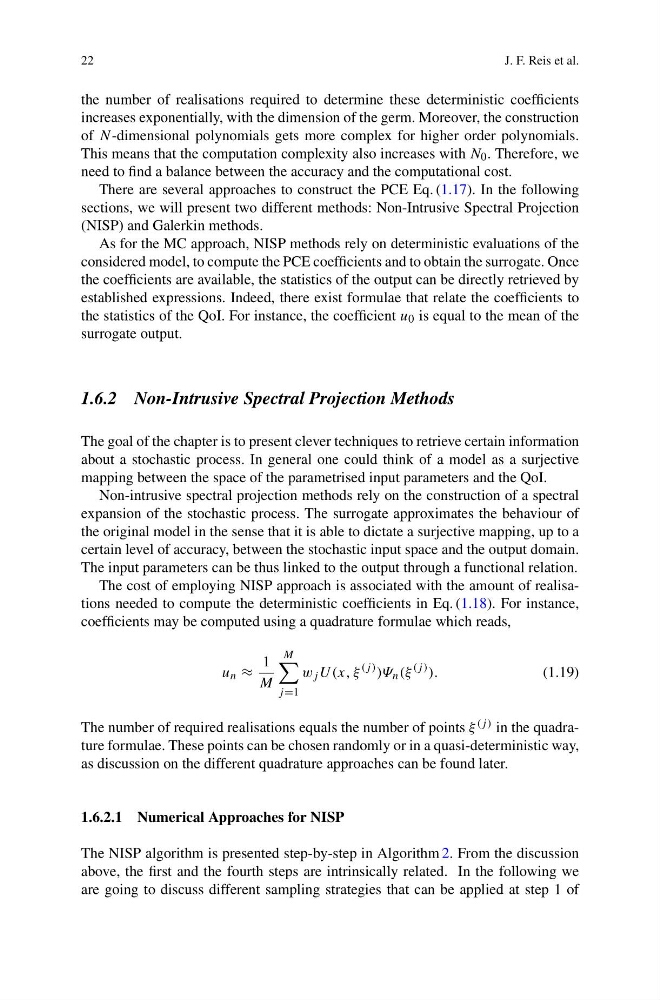
The cost of employing NISP approach is associated with the amount of realisations needed to compute the deterministic coefficients in Eq. (1.18). For instance,
coefficients may be computed using a quadrature formulae which reads,
u n ≈
1
M
M
j =1
w j U(x, ξ
(j ) )Ψ n (ξ
(j ) ).
(1.19)
The number of required realisations equals the number of points ξ (j ) in the quadrature formulae. These points can be chosen randomly or in a quasi-deterministic way,
as discussion on the different quadrature approaches can be found later.
1.6.2.1 Numerical Approaches for NISP
The NISP algorithm is presented step-by-step in Algorithm 2. From the discussion
above, the first and the fourth steps are intrinsically related. In the following we
are going to discuss different sampling strategies that can be applied at step 1 of
J. F. Reis et al.
the number of realisations required to determine these deterministic coefficients
increases exponentially, with the dimension of the germ. Moreover, the construction
of N-dimensional polynomials gets more complex for higher order polynomials.
This means that the computation complexity also increases with N 0 . Therefore, we
need to find a balance between the accuracy and the computational cost.
There are several approaches to construct the PCE Eq. (1.17). In the following
sections, we will present two different methods: Non-Intrusive Spectral Projection
(NISP) and Galerkin methods.
As for the MC approach, NISP methods rely on deterministic evaluations of the
considered model, to compute the PCE coefficients and to obtain the surrogate. Once
the coefficients are available, the statistics of the output can be directly retrieved by
established expressions. Indeed, there exist formulae that relate the coefficients to
the statistics of the QoI. For instance, the coefficient u 0 is equal to the mean of the
surrogate output.
1.6.2 Non-Intrusive Spectral Projection Methods
The goal of the chapter is to present clever techniques to retrieve certain information
about a stochastic process. In general one could think of a model as a surjective
mapping between the space of the parametrised input parameters and the QoI.
Non-intrusive spectral projection methods rely on the construction of a spectral
expansion of the stochastic process. The surrogate approximates the behaviour of
the original model in the sense that it is able to dictate a surjective mapping, up to a
certain level of accuracy, between the stochastic input space and the output domain.
The input parameters can be thus linked to the output through a functional relation.
The cost of employing NISP approach is associated with the amount of realisations needed to compute the deterministic coefficients in Eq. (1.18). For instance,
coefficients may be computed using a quadrature formulae which reads,
u n ≈
1
M
M
j =1
w j U(x, ξ
(j ) )Ψ n (ξ
(j ) ).
(1.19)
The number of required realisations equals the number of points ξ (j ) in the quadrature formulae. These points can be chosen randomly or in a quasi-deterministic way,
as discussion on the different quadrature approaches can be found later.
1.6.2.1 Numerical Approaches for NISP
The NISP algorithm is presented step-by-step in Algorithm 2. From the discussion
above, the first and the fourth steps are intrinsically related. In the following we
are going to discuss different sampling strategies that can be applied at step 1 of